
More Information
Submitted: 21 October 2019 | Approved: 03 December 2019 | Published: 04 December 2019
How to cite this article: Panahinia R, Behnia S. Bio-moleculear thermal oscillator and constant heat current source. Int J Phys Res Appl. 2019; 2: 051-055.
DOI: 10.29328/journal.ijpra.1001016
Copyright License: © 2019 Panahinia R, et al. This is an open access article distributed under the Creative Commons Attribution License, which permits unrestricted use, distribution, and reproduction in any medium, provided the original work is properly cited.
Keywords: DNA; Phononics; Thermal oscillator; Constant heat current source; Power spectrum; Thermal conductivity

Bio-moleculear thermal oscillator and constant heat current source
R Panahinia* and S Behnia
Department of Physics, Urmia University of Technology, Urmia, Iran
*Address for Correspondence: Robabeh Panahinia, Urmia University of Technology, Urmia, Iran, Tel: +984433686249; Email: [email protected]
The demand for materials and devices that are capable of controlling heat flux has attracted many interests due to desire to attain new sources of energy and on-chip cooling. Excellent properties of DNA make it as an interesting nanomaterial in future technologies. In this paper, we aim to investigate the thermal flow through two sequence combinations of DNA, e.g, (AT)4 (CG)4 (AT)4 (CG)4 and (CG)8 (AT)8. Two interesting phenomena have been observed respectively. In the first configuration, an oscillatory thermal flux is observed. In this way, an oscillating heat flux from a stationary spatial thermal gradient is provided by varying the gate temperature. In the second configuration, the system behaves as a constant heat current source. The physical mechanism behind each phenomenon is identified. In the first case, it was shown that the transition between thermal positive conductance and negative differential conductance implies oscillatory heat current. In the latter, the discordance between the phonon bands of the two coupled sequences results in constant thermal flow despite of increasing in temperature gradient.
The Recent decade has been faced with the great research interests in heat flow management in nano scale devices [1,2]. The ability to thermal control may have interesting applications such as heat waste recovery, energy storage, and phononics. In the phononics (understanding and controlling the thermal flow), it is desirable to develop the thermal circuit ingredients, such as thermal diodes [3-5], thermal transistors [6,7], thermal memory [8] and thermal logic gate [9], analogous to electrical circuit components. The first report of heat manipulation was represented in 2002 [3]. It was an elementary presentation of nano thermal diode or rectifier. In 2006, Li, et al. demonstrated the first model of thermal transistor [6]. It was a three-gate system in which by tuning the temperature of the third gate, one can manage the thermal current in the two gates.
Moreover, constant current sources and current oscillators, which have the significant roles in electronic circuits, have been founded for many years. Their thermal peer, namely, heat current oscillators and constant heat current sources are poorly realized. Thermal oscillator provides the oscillatory thermal current from a stationary temperature bias. While, a steady heat current source prepares a constant thermal flow contrary to a variation in the temperature bias. They are two main bases of phononics.
The purposes of the current paper are two folds. First, a thermal oscillator for creating an oscillating heat flux from a stationary spatial temperature gradient between a hot reservoir and a cold reservoir is suggested. Second, a new design of constant thermal current sources is presented.
In the first part, the system configuration includes two portion, e.g. “Source” (S) and “Drain” (D). At the right end, there is a hot reservoir and the cold reservoir is at the left end. The source and drains are attached to each other. The source is joined to the hot reservoir from right. Drain is connected to the cold reservoir from left. At the interface, the system is coupled to the gate reservoir. The gate reservoir play the role of control thermostat equilibrated at TG. The configuration is shown in figure 1. Each portion includes an asymmetric sequence combination of DNA molecule. Superior attributes of DNA propose employing it as an outstanding nanomaterial in future technologies. DNA molecule benefits from high mechanical flexibility, so it will not be imposed any break down during an operation.
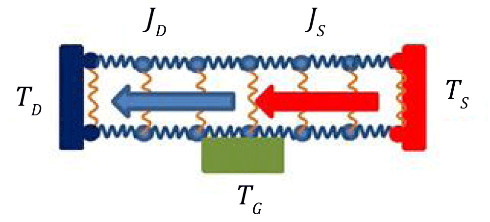
Figure 1: Schematic representation of thermal oscillator.
Many efforts as much as mathematical models have been devoted to characterize DNA dynamic [10]. It is stated that Peyrard-Bishop-Daxois model (PBD) can successfully describe DNA dynamics [11-13]. In this model, the strong covalent bonds were utilized to describe the nucleotides which are aligned in the same strand. An anharmonic nearest-neighbor interactions demonstrates the covalent bonds. A nonlinear on-site potential is employed to characterize the coupled strands through the weak hydrogen bonds.
The Hamiltonian of the model writes
H = HD + HS (1)
Such that
wherein, is the on-site Morse potential. The Morse potential illustrates the transverse fluctuations of the hydrogen bonds connecting complementary bases. The described potential by
represents the stacking interactions.
yn demonstrates the fluctuation of base pairs through the hydrogen bonds and m represents the reduced mass of a base pair.
Parameters of the model reads as: Dn = 0.05 eV for AT base pairs, Dn = 0.075 eV for CG base pairs.
for n = 1,..., N.
The equations of motion for each base pair is described as
When a system is connected to the heat baths at different temperatures, one can consider the heat transport characteristics in a Hamiltonian system at a stationary state. Various models have been employed to control the temperature of the system as a thermostat, e.g, the Anderson thermostat [14], Berendsen thermostat [15], Nos´e-Hoover thermostat [16], and Langevin thermostat [17]. In the Langevin approach, the heat bath is modeled by using the stochastic process, so the reservoirs is simulated by adding a dissipative term and a stochastic Gaussian white noise term in the Newtonian equation of motion. Due to stochastic nature of Langevin heat bath, its utilization is accompanied by complication and consuming. To prevail the difficulties originated from stochastic processes, a new approach is developed by Nose and Hoover with a deterministic nature. It includes only one imaginary variable. This variable simulates system’s achieve to desired temperature. It is known that in the nearly linear chains, Nos´e-Hoover thermostat is not effective and will result to artificial results [18,19]. In such cases, it is essential to use Langevin approach despite of its difficulties. Fortunately, DNA has a strong nonlinear nature and one can use the Nose-Hoover approach with confident.
Now, we thermalize the r first particles at TR and l last particles at TL and g intermediate particles at TG by using Nose-Hoover thermostat chains [16]. The dynamic of thermostats is described as:
So, the dynamic of each bas pair is represented by:
where n = 1, 2, ..., N and r,s,g respectively show the left, right, and gate thermostats. By defining the new variable the N equations (1) degrades to 2N coupled ordinary differential equations as:
Where, fn demonstrates the right hand side of equation (1). ODE45 solver is used to integrate the differential equations of motion. To reach the steady state, long enough time is regarded. Local temperature at site n is computed by Virial theorem:
By using the continuity equation for the energy density
One can write the local heat flux as:
So, the total heat flux is defined as . High enough time (200 ns) is regarded so that the system attains to the steady state. Figure 2 shows the steady state flow of heat flux through a homogenous chain (AT) after 2 × 10⁷ tu.
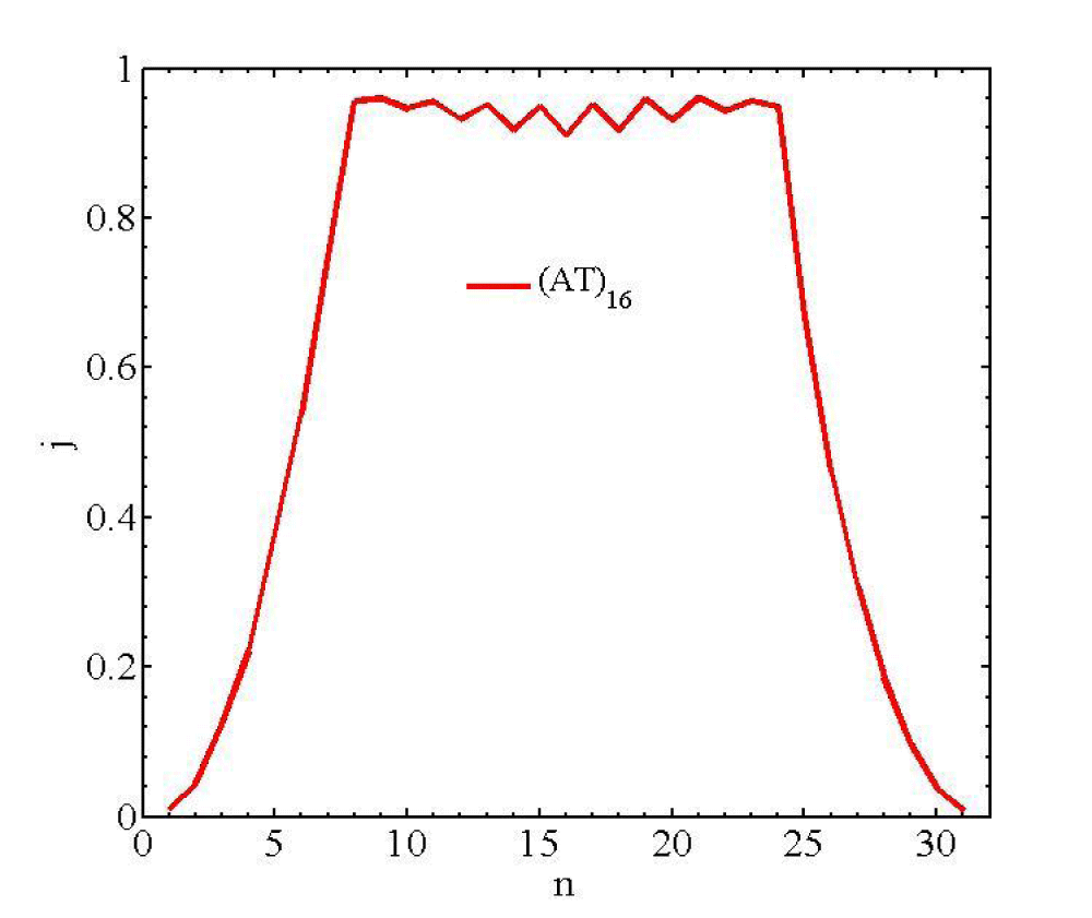
Figure 2: Shows the steady state flow of heat flux through a homogenous chain (AT) after 2 × 10⁷ tu.
Thermal oscillator
An electronic relaxation oscillator creates an oscillating electronic current from a stationary spatial voltage. Thermal analogue of electronic oscillator is desirable for technological application like energy harvesting devices, switching devices or clocking devices and sensing devices. A few reports of thermal oscillator have been presented based on different mechanisms (Ref. 20 and references therein). Here, it was shown that the phase transition between the positive differential thermal conductivity and negative differential thermal conductivity is responsible to thermal oscillation mechanism. The system is configured as follows: two coupled chain are the same, each one with the sequence (AT)4 (CG)4. The system at the left end is attached to the cold thermostat at TC = 3 K. At the middle part, the chain is coupled to the gate thermostat as a control thermostat. The hot thermostat is connected to right end which is equilibrated at TH = 30 K. Figure 3 shows the oscillating heat current through two S and D segments. To consider the physical nature of phenomenon, we calculate the thermal
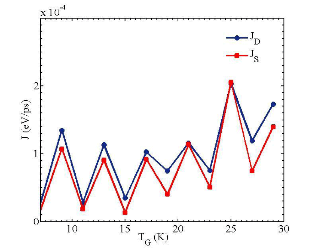
Figure 3: The oscillation of heat current in the fixed temperature bias.
Figure 2 shows local heat flux jn through the system after 2 × 10⁷ tu conductivity through the Fourier’s law. The Fourier’s law is expressed as
where the heat flux j is the amount of transported heat through the unit surface per unit time. ∇T is ×% the temperature gradient.
It was shown that the transition between positive differential thermal conductivity and negative differential thermal conductivity implies oscillatory heat current. It is proved that negative differential thermal conductivity is possible due to nonlinear nature of system. Nonlinearity varies the phonon band’s position with temperature. It makes phonon bands have match and mismatch dependent on temperature [6,21]. The result is shown in figure 4.
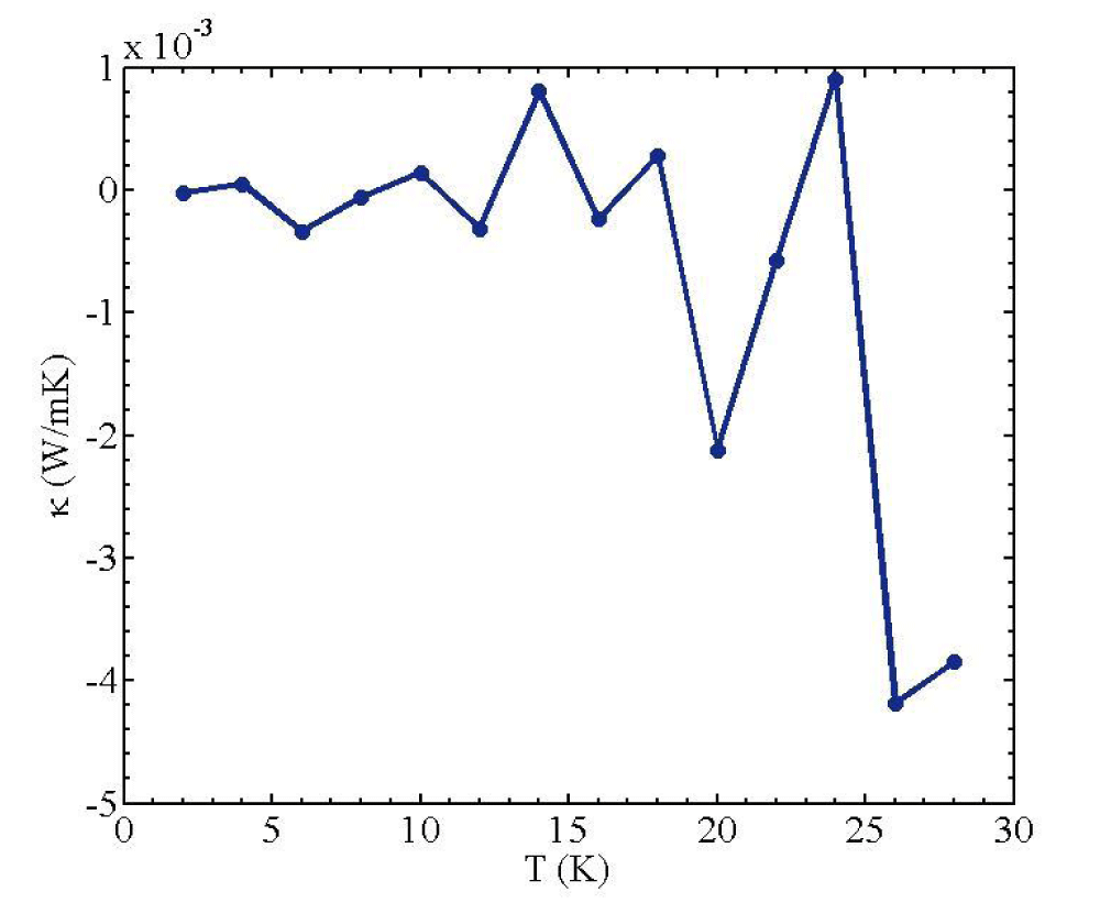
Figure 4: Phase change between positive differential thermal conductivity and negative differential thermal conductivity.
Constant heat current source
Constant current sources have been employed in electronic circuits for many years. A constant (electric) current source supplies a fixed charge flow, in spite of a variation in the power supply. In Ref. 22, by attaining complete NDTR, it has been presented the first report of constant thermal current sources. Here we present new design of constant thermal current sources. The chain comprises of 32 base pairs. Sequence combination (CG)8 (AT)8 is used. The left end is coupled to the cold thermostat at 2 K. The right end is connected to the hot thermostat equilibrated at 20 K. It was shown that by varying right temperature, the thermal current in the sequence is nearly constant. The result is shown in figure 5. Under presented situation, the device can suffer the changes of the temperatures of heat baths and yields a fully stable value of heat current.
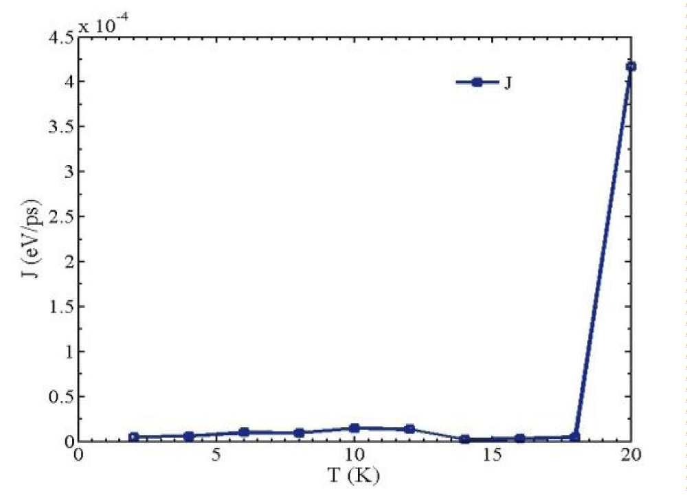
Figure 5: Constant heat current source despite of increasing temperature bias.
To investigate the mechanism which is resulted in occurrence of constant current source, we consider the power spectrum of AT and CG segments. The temperature of CG sequence (blue) is fixed at 2 K. The temperature of AT sequence is increasing T+ = T- (1 + ∇). For AT sequence, power spectrums have been illustrated as a pink (18 K) and red (10 K) style in the figure 6a,b. For CG sequence which is equilibrated at 2 K, power spectrum is shown as a blue style.
Clearly it was seen from figure 6 that the discordance between the phonon power spectrums of the two attached sequences results in constant thermal flow despite of increasing in temperature gradient. Moreover, it is obvious that by increasing the temperature of AT sequence e.g., by increasing the temperature difference, the overlap between phonon bands do not vary.
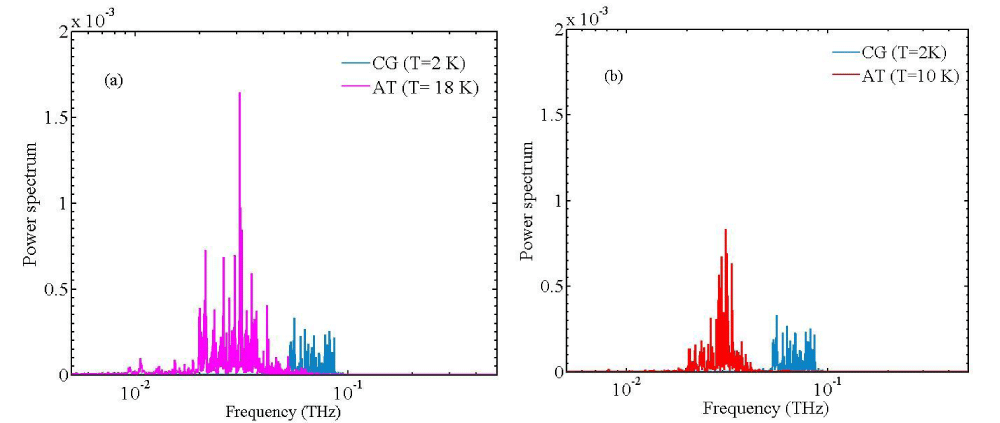
Figure 6: Power spectrum of CG at 2 K and power spectrum of AT sequence at (a) 18 K, (b) 10 K
So, in the region determined at the figure 5, the thermal current through the system is constant. The temperature profile is shown in figure 7. It is clear the heat flux could not flow from first half part of the sequence to the left part. So, one can use this property to design the constant thermal source.
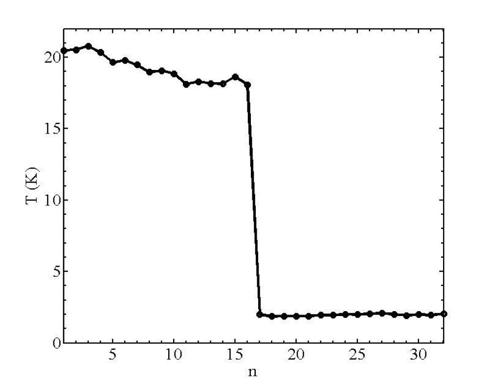
Figure 7: Temperature profile of a DNA sequence with sequence combination (AT)4/(VG)4.
Thermal management in nanodevices may have a fundamental role in the development of future nanoelectronic circuits due to the importance of the heat among nanoelements. Self-assembly capabilities and elastic properties of DNA make it as foremost nanowire materials. Ability of DNA for coding, prediction and its intrinsic diversity persuade one to construct the electronic and heattronic devices based on DNA. We proposed a model of the thermal oscillator and constant heat current source based on DNA nano wire. The underlying physical mechanisms of such behaviors are determined. It was shown that the change in material state between conducting and negative conducting phases is responsible for oscillation of heat current. Also, it was shown that the inconformity between the power spectrum of the two interface particles in some temperature range make constant heat current source and possible.
- Maldovan M. Sound and heat revolutions in phononics. Nature. 2013; 503: 209-217. PubMed: https://www.ncbi.nlm.nih.gov/pubmed/24226887
- Wang L, Li B. Thermal memory: a storage of phononic information. Phys World. 2008; 21: 27.
- Terraneo M, Peyrard M, Casati G. Controlling the Energy Flow in Nonlinear Lattices: A Model for a Thermal Rectifier. Phys Rev Lett. 2002; 88: 094302.
- Yang N, Gang Z, Li B. Carbon nanocone: A promising thermal rectifier. App Phys Lett. 2008; 93: 243111.
- Tian H1, Xie D, Yang Y, Ren TL, Zhang G, et al. A novel solid-state thermal rectifier based on reduced graphene oxide. Sci Rep. 2012; 2: 523 PubMed: https://www.ncbi.nlm.nih.gov/pubmed/22826801
- Li B, Wang L, Casati G. Negative differential thermal resistance and thermal transistor. App Phys Lett. 2006; 88: 143501.
- Mendonca MS, Pereira E. Effective approach for anharmonic chains of oscillators: Analytical description of negative differential thermal resistance. Phys Lett A. 2015; 379: 1983-1989. PubMed:
- Wang L, Li B. Thermal Memory: A Storage of Phononic Information. Phys Rev Lett. 208; 101: 267203.
- Wang L, Li B. Thermal Logic Gates: Computation with Phonons. Phys Rev Lett. 2007; 99: 177208.
- Yakushevich LV. Nonlinear physics of DNA. John Wiley & Sons. 2006.
- Dauxois T, Peyrard M, Bishop AR. Entropy-driven DNA denaturation. Phys Rev E. 1993; 47: R44.
- Voulgarakis NK, Redondo A, Bishop AR, Rasmussen KØ. Probing the Mechanical Unzipping of DNA. Phys Rev Lett. 2006; 96: 248101
- Weber G, Jonathan WE, Neylon C. Nat Phys. 2009; 5: 769.
- Karakare S, Kar A, Kumar A, Chakraborty S. Patterning nanoscale flow vortices in nanochannels with patterned substrates. Phys Rev E. 2010; 81: 016324.
- Lemak AS, Balabaev NK. On The Berendsen Thermostat. Mol Sim.1994; 13: 177-187.
- Hoover WG. Canonical dynamics: Equilibrium phase-space distributions. Phys Rev A. 1985; 31: 1695.
- Dhar A. Heat transport in low-dimensional systems. Adv Phys. 2008; 57: 457-537.
- Savin AV, Gendelman OV. Heat conduction in one-dimensional lattices with on-site potential. Phys Rev E. 2003; 67: 041205.
- Dhar A. Comment on “Can Disorder Induce a Finite Thermal Conductivity in 1D Lattices?” Phys Rev Lett. 2001; 87: 069401.
- Gotsmann B, Menges F. US. Patent. 2016L; 20,160,112,050.
- Behnia S, Panahinia R. Designing thermal diode and heat pump based on DNA nanowire: Multifractal approach. Phys Lett A. 2017; 381: 2077-2084.
- Wu J, Wang L, Li B. Heat current limiter and constant heat current source. Phys Rev E. 2012; 85: 061112.