
More Information
Submitted: 28 January, 2020 | Approved: 06 March 2020 | Published: 09 March 2020
How to cite this article: Golam Sarwar ATM, Khan MR, Khan A. A quantum mechanical model for hole transport through DNA: predicting conditions for oscillatory/non-oscillatory behavior. Int J Phys Res Appl. 2020; 3: 046-057.
DOI: 10.29328/journal.ijpra.1001022
Copyright License: © 2020 Golam Sarwar ATM, et al. This is an open access article distributed under the Creative Commons Attribution License, which permits unrestricted use, distribution, and reproduction in any medium, provided the original work is properly cited.

A quantum mechanical model for hole transport through DNA: predicting conditions for oscillatory/non-oscillatory behavior
ATM Golam Sarwar1, M Rezwan Khan1 and Arshad Khan2*
1Department of Electrical and Electronic Engineering, United International University, Dhaka, Bangladesh
2Chemistry Department, The Pennsylvania State University, USA
*Address for Correspondence: Arshad Khan, Chemistry Department, The Pennsylvania State University, USA, Tel: (814) 375-4744; Email: [email protected]
A quantum mechanical model that considers tunneling and inelastic scattering has been applied to explain the hole transfer reaction from a G (Guanine) base to a GGG base cluster through a barrier of Adenine bases, (A)n (n = 1-16). For n = 1, the ratio of tunneling to inelastic scattering is about 6, which is sharply decreased to around 0.23 and 5.23 × 10⁻⁸ for n = 4 and 16 respectively, suggesting dominance of inelastic scattering for n ≥ 4. As in experiment, the calculated product yield ratios (PGGG) exhibit a strong distance dependence for n < 4, and a weak distance dependence for n ≥ 4. We also predict conditions under which oscillatory or non-oscillatory charge transfer (CT) yield are expected.
Charge transport (CT) through DNA is an important topic of recent interest and has biological significance as oxidation of a base forms a hole (positive charge) and initiates its transport from one base to a distant base, and hence, may result in mutations and carcinogenesis [1]. It is also important in the area of nanotechnology where researchers are trying to develop a highly conducting molecular wire with DNA [2-6]. Recently, it was shown theoretically that certain substituent groups attached to DNA bases can lower its activation energy barrier for hole transfer reaction, and hence, can enhance its conductivity [7]. Because of these potential applications in the field of molecular biology as well as materials science, significant amount of experimental [8-15] and theoretical studies [16-21] have been carried out on DNA and related systems [15] in order to understand the hole transport phenomenon. The experimental studies applied techniques like fluorescence quenching of the donor (as in ref.9) molecules, analysis of the strand cleavage products of DNA (as in ref.14), and cyclic voltammetry [15] for single and double stranded peptide nucleic acids. The experimental results are usually interpreted in terms of the following classical expression that relates the rate of CT (kCT) to donor acceptor distance (R):
kCT = ko exp (-βR) (1)
Here, ko is the pre-exponential factor, and β is the falloff parameter with a value ranging from around 0.1 to 1 Å-1. While a large β value (close to 1) indicates a strong distance dependence of the CT rate, a small value indicates weak distance dependence. Grozema, et al. [17e] examined a correlation between the ionization energy (IE) difference between the donor and the bridge (barrier) and the β value, and have noticed that as the IE difference is increased the β value is also increased. For hole transfer from a G base to an acceptor through the intervening A bases (IE difference = 0.55 ev), this model predicts a fairly large β value of 0.85 Å-1 (eq 1), and hence, suggests a tunneling mechanism. As the IE difference together with the β value gets significantly smaller, the charge is considered to become delocalized within the bridge and the mechanism is changed from the single-step tunneling to the molecular wire type. Thus, for a large β value and IE difference, as in G(A)nGGG system, only a strong distance dependence, and hence, tunneling is expected as a hole transfer mechanism. Giese, et al. [13], experiment, however, suggests a strong distance dependence followed by a weak distance dependence as n value is increased, even when the same IE difference is maintained between the donor and the bridge. In their experiment, the hole-water reaction products (P) are determined at different base sites for the G(A)nGGG base sequence with n = 1-16. Each G represents a GC (Guanine-Cytosine) base pair and A represents an AT (Adenine-Thymine) base pair. The experimental [13] product yield ratios (PGGG) exhibit a strong distance dependence for n < 4, and a weak distance dependence for n ≥ 4. Giese, et al. [13], explain their experimental results by considering tunneling for n < 4, that switches to hopping through A bases (A-hopping) for n ≥ 4. There are quite a number of researchers [16b,17e,20,21] who have proposed a similar change in mechanism at around n = 4 for DNA and related systems [15]. In spite of all these research efforts to explain the hole transport phenomenon together with its characteristic strong and weak distance dependence, as of today there is no generally accepted CT mechanism for all n values. Even though there is a consensus regarding the operation of a tunneling mechanism for small n values [16g], disagreements exist in explaining the weak distance dependence at large n values. Mechanisms like hopping [16g] or “molecular wire” type [10g] are often considered for n ≥ 4. A “molecular wire” mechanism [10g] involves strongly coupled donor-acceptor system, and the CT takes place through π electrons according to band-like transport mechanism. The second mechanism, as discussed above, is an incoherent hopping [16g] mechanism where charge hops between base pairs until it reaches the acceptor. No matter whether a hopping or molecular-wire type transmission is considered for large n values, a change of mechanism from tunneling has been considered at n = 4. A recent molecular dynamics (MD) study [22] however, contradicts this suggestion of mechanism change at a particular n value (n = 4) as product formation was noticed within the A bases even for n = 2, at which coherent tunneling was considered to be the only mechanism. In order to account for their findings, the authors [22] assumed simultaneous operation of tunneling and hopping mechanisms. Although hopping has been considered by quite a few researchers to explain the weak distance dependence, the validity of hopping has been questioned on the basis of certain experimental results [23]. Similarly, the band-like hole transmission [10g] (molecular wire mechanism) is expected to give much larger product concentration within the A bases (barrier) than what has been observed in experiments [13].
Two other important aspects that any CT model needs to address are oscillatory nature of CT yield [8] and charge delocalization [24], which have been observed in recent experiments. O’Neill and Barton’s [8] experiments suggest an oscillatory CT yield with an increased number of A bases in Ap*(A)nG base sequence, where Ap* represents a photo-excited 2-aminopurine (Ap*) bonded to a T base. This result is quite different from that of Giese and co-workers where the CT yield is non-oscillatory [13]. So far, no explanation has been provided for the oscillatory/non-oscillatory nature of CT yield, and hence, required additional studies.
A polaron model [21] incorporates some degree of charge delocalization and describes CT in terms of hopping between polaron sites. Although a drift of polarons (charge carrier) with accompanying polarization of the medium surrounding the DNA can explain the weak distance dependence for n > 3, it fails to account for strong distance dependence for n < 4 [23].
The research of various authors, discussed above, certainly indicates controversy rather than agreement on various DNA CT aspects. A number of questions can be raised regarding the CT phenomenon that we know today. What is the true nature of the CT mechanism; tunneling and hopping, tunneling and molecular wire-like transmission, or tunneling and altogether a different second mechanism? Also, do these mechanisms operate simultaneously at every n value or is there an onset of the second mechanism at n = 4? Besides, when would one expect oscillatory or non-oscillatory CT yield? In order to find answers to above questions the present theoretical study has been undertaken. Herein, we primarily focus on the issue of charge delocalization, CT mechanism and product formation at different base sites (in G(A)nGGG structure) and the origin of oscillatory behavior that has been reported earlier [8]. This study is different from most other theoretical studies[16] in the sense that no change in CT mechanism is assumed a priori at any n value; rather, the hole transmission through the G(A)nGGG base sequence is considered to be due to both tunneling and inelastic scattering that takes place simultaneously. It should be mentioned that the inelastic scattering is an expected phenomenon for a moving hole from its donor (G or Ap*) site to an acceptor site (GGG or G) through intervening A bases. This paper has been divided into several segments. First, we develop the CT mechanism, calculate product concentrations at different base sites, and at the end, provide conditions under which one can expect the oscillatory or non-oscillatory CT yield.
Simplified 1D potential diagram for hole transportation
The most common practice in electron transportation phenomenon in solid state physics is the consideration of effective mass approximation. In any periodic structure the effective mass approximation allows one to eliminate the periodic potential variation with distance and replace it by a flat potential profile. When one type of material forms a bond with another type, the energy profile for each type can be considered to be flat and a potential discontinuity is expected at the interface. In this theoretical study a DNA molecular chain is considered with a G base separated from a GGG base cluster by a number of A bases (1-16) that form an energy barrier as shown in figure 1. In this figure potential energy values on the far left and far right are assumed to be very large implying that there is no CT from the side chains. This assumption is quite consistent with the fact that each DNA base is bonded to the side chain via a deoxyribose sugar unit that has a large ionization potential (10.5 ev) [25]. However, the barrier on the immediate right side of the lone G is finite (0.73 ev) [26] and is made up of A bases which the transporting hole from G to GGG will experience, and has been obtained from the calculated reorganization energy values [26]. While experiments do not provide a barrier height value for the hole transfer reaction, a significant fall in the CT rate with the number of intervening A bases suggests the presence of an energy barrier [13]. In addition, the reorganization energy values deduced from experimental rates [27] show an excellent agreement with the calculated values suggesting an accurately calculated reorganization energy values and hence, the value of the barrier height [26].
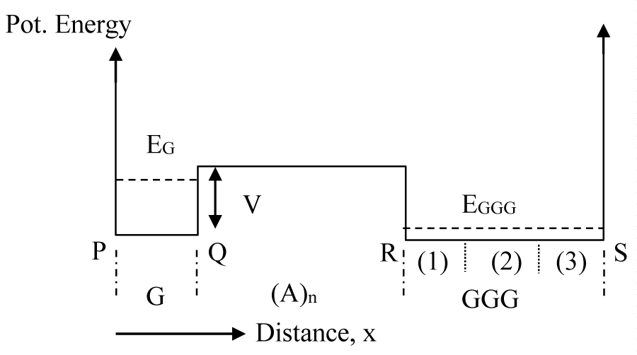
Figure 1: Schematic potential energy diagram for the DNA base sequence, G(A)nGGG. Bottom of the potential well is assumed to be at zero potential and the barrier height to be V. The numbers (1), (2) and (3) show the locations of three G bases of the GGG cluster.
Before developing our QM CT model in details, we provide a physical picture of the model that involves the DNA structure of figure 1. As soon as a hole is formed on the G base (by loss of an electron) it remains confined within the base for a brief period of time. The wavefunction of this newly formed hole (ψ0) then gradually tunnels to GGG through the finite barrier width of (A)n bases (n = 1,2,3, etc.) and forms a distributed wavefunction (ψ1) throughout the potential structure of figure 1. Simultaneously, however, there takes place another phenomenon called “inelastic scattering” due to interaction of the hole with the vibrating atoms of the bases. Through such interaction the hole attains enough energy to move above the barrier, and hence, can flow directly from G to GGG. As the GGG potential well is three times wider, its energy states are much lower than that of the G. After a certain time interval from the creation of the hole, it totally vanishes from its upper state and finally, appears in the lower most state (ψ2). Any reverse scattering from the lower most state to a higher energy state is quite unlikely due to a large energy gap.
So, in this paper, we first calculate the initial localized wavefunction (ψ0) when the hole is created and its expected life-time (τ1) required for it to delocalize within all the bases of the G(A)nGGG sequence. Then we calculate this delocalized wavefunction (ψ1) and its life time (τ2), after which transition to the lower most state (ψ2) takes place. It is expected that some products will be formed in each energy state (ψ0, ψ1 and ψ2) with a spatial distribution corresponding to the probability density function (wavefunction squared).
As the potential energy diagram depicted in figure 1 is a simplified 1D potential well, we applied the following Schrodinger Equation in 1D formulation:
(1a)
The corresponding equation for the probability current density is given by
(1b)
Here, m is the effective mass of the hole, ψ is its wavefunction for the energy state E, and V is the potential energy. The above equation is a steady state equation when there is no change in particle energy, and under a bound condition of figure 1 potential there cannot be any probability current S in any direction. If we assume that after the formation of a hole at the lone G site its wavefunction interacts with the A bases in the barrier and the remote GGG base cluster, the solution will no longer remain as a time invariant one. A time dependent Schrodinger Equation is a complicated one to solve, for which we applied the following simple mathematical treatment after the consideration of three different hole states (initial, intermediate and final states, discussed in section 2.4). If any portion of the wavefunction interacts with the vibrating atoms of bases (referred to as inelastic scattering) and changes its original energy state, the probability of the existence of the hole in that particular state will gradually decrease. In order to include this effect, an imaginary quantity is introduced in the (E-V) term of equation (1a) to yield eqn (2).
(2)
Here, i is the imaginary quantity and Vi is the newly introduced term in the equation. The Vi term can be treated either as a component of an imaginary energy or an imaginary potential. Whatever the choice is, the final equation remains the same. It may be noted that the imaginary potential term Vi is a function of temperature [28,29] as the molecular vibrations or even chemical reaction rates can vary with temperature. So, it is possible to address the temperature variation by making Vi as a function of temperature. For any given energy E of the hole, the functional forms of the wavefunction in different regions (Figure 1) are given below:
(3)
Where γ = for region PQ
= for region QR
= for region RS
Here V is the height of the potential barrier and m1, m2 and m3 are the effective mass in PQ, QR and RS region (Figure 1) respectively. Vi2 and Vi3 are the imaginary potential in QR and RS regions respectively. Inelastic scattering in region PQ is ignored (Vi1 = 0). The usual solution technique of Schrodinger’s equation for such a potential structure involves application of boundary conditions at each potential discontinuity and evaluation of ‘C’s and ‘D’s for each region of a normalized wavefunction distribution. We used the technique presented in [30,31] to find out the eigenenergy and normalized wavefunction. The technique presented in [31] is particularly useful to evaluate normalized wave functions in presence of imaginary potentials. Once the wavefunction is known, the probability current density S (eqn.1b) can be easily calculated at any position using the form of solution presented in eqn. (3).
After the imaginary potential term is introduced within the A and GGG regions, the values of γ (eq.3) become complex resulting in gradual decay of the wave function in those regions due to inelastic scattering. If we represent the time constant of wave function decay as τi, then we can write
(4)
Here, SQ is the probability current density at location Q (Figure 1) and has been defined by the number of holes being transferred per unit time. If such a process continues, after a while, the total wave function from the well at G will vanish and the hole will disappear from G and make a transition to GGG. No backward transition is considered as the initial energy at G is much higher than that at GGG [32].
Deriving equations for product concentrations at different base sites
Whenever a hole is formed at the lone G base, it has a very high energy barrier on its left hand side and the probability that the hole will cross that barrier is almost nil (Figure 1). The barrier on the right hand side is much smaller with a height of around 0.73 ev [26], and the hole may tunnel through that barrier or may have sufficient energy exchange with its neighboring bases due to thermal vibration or phononic interaction to overcome the barrier, and move to the GGG region. The tunneling through the barrier is a coherent process and there is no change in energy. On the other hand, if we consider an energy interchange with the surrounding molecules, there is a change in energy of the hole and a coherent process cannot be assumed. However, due to finite probability of both the processes, they would occur simultaneously and the ultimate result is the combined effect of both the tunneling and inelastic scattering. Hence, it can be concluded that a hole generated at the G site will die out from that state and have the probability of reappearing in some other state at some other location. It is a well-known QM phenomenon that the energy states go lower as the width of a quantum well gets larger. This situation is depicted in figure 1 by indicating EG to be much higher in energy than EGGG. Once the hole leaves its original energy state EG, it will have a high probability of appearing in a lower energy state like EGGG. As mentioned above, in calculating product concentrations at different base sites, we considered the following three hole-states that contribute to product formation.
Product formation during initial hole state
As soon as a hole is formed at the G site, its wave function (ψ0) is primarily localized onto it with some penetration into the barrier on the right as shown in figure 2a. This is a metastable condition, and it is expected that the metastable wave function (ψ0) will tunnel through the barrier (Figure 2b) and elastically transform to the wave function ψ1 (Figure 3), which the wave function is corresponding to the whole potential structure. The time required for such a transformation is the time required for the accumulation of wavefunction ψ1 in GGG. If the probability current density at R (Figure 1) for this state (ψ0) is SR0 then, the time constant (τ1) for such a process to buildup ψ1 in GGG is given by
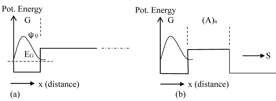
Figure 2: (a) The eigenenergy and eigenfunction of the initial hole state at G when the hole is created. (b) The leakage of the wave function through the barrier after the creation of the hole.
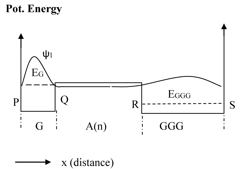
Figure 3: The potential energy diagram applied to calculate the hole state after time τ1. The schematic wave function for the structure is shown as ψ1 corresponding to the energy EG.
(5)
If we assume that the probability of product formation rate at any location is directly proportional to the probability of hole existence (includes hole formation and decay) in that location and inversely proportional to the reaction time then
PG0 = B αG0 τC0 (1- exp(-τ1 /τC0))/τGC (6a)
PA0 = B αA0 τC0 (1-exp(-τ1 /τC0))/τAC (6b)
PGGG0 = B αGGG0 τC0 (1-exp(-τ1 /τC0))/τGGGC (6c)
Here τXC is the reaction time in the region X (region for G, A or GGG in figure 1) and τC0 is the mean reaction time for the entire structure (Figure 1) calculated by taking the weighted average of reaction rates (inverse of reaction time) in different regions (please see Appendix 1 for a detailed derivation). The proportionality constant B takes into account any variation in the probability of existence of the wave function in the energy state under consideration and has the value of unity in this case as the hole is originated at this state. The αXj represents the probability of hole formation at a particular site and is calculated from the normalized wavefunction over the region X by applying the following eqn:
(6d)
Here, X represents the region (G, A or GGG) and j is the subscript for the wave function under consideration. If we consider X to be the region for G and set j = 0, then eqn. 6d gives a value for αG0 obtained by integrating the square of the wave function ψ0 over the region of G (PQ in figure 1). Other values of α, defined later in eqns 8 and 10, are also calculated in a similar manner. For a quick check of the formula 6a-c, when τ1 or life-time of the hole is zero, PG0= 0, that is, life time of the hole is too short for that energy state to form any product. On the other hand, when τGC (reaction time) is infinity or when the reaction takes place very slowly compared to other regions, again PG0= 0. As expected, in this situation the hole does not exist at the base site long enough to form any product.
When the product formation probability due to ψ0 at different base sites are known from eqns 6a-c, the total probability (for initial hole state) is given by
P0= PG0+ PA0+ PGGG0 (7)
Product formation during intermediate hole state
Now, the product formation probabilities at G, A and GGG sites together with the total probability (P1) are given as follows, similar to eqn. 6a, 6b and 6c, for the hole state defined by ψ1:
PG1 = (1-P0) αG1 τC1 (1- exp(-τ2 /τC1))/τGC (8a)
PA1 = (1-P0) αA1 τC1 (1-exp(-τ2 /τC1))/τAC (8b)
PGGG1 = (1-P0) αGGG1 τC1 (1-exp(-τ2 /τC1))/τGGGC (8c)
P1= PG1+ PA1+ PGGG1 (9)
As described earlier, α values are calculated by applying eq.6d with j = 1 for different regions of bases. Here (1-P0) = B, as defined in eqns 6a-c and eqns in Appendix 1, and P00.
Product formation during final hole state and total quantities
As a result of inelastic scattering the hole finally makes a transition to the lowest energy state, EGGG. Figure 4 shows the schematic potential energy diagram along with the probability distribution function for the final hole state represented by ψ2.
PG2 = (1-P0-P1) αG2 τC2 (1- exp(-τ3/τC2))/τGC (10a)
PA2 = (1-P0-P1) αA2 τC2 (1-exp(-τ3 /τC2))/τAC (10b)
PGGG2 = (1-P0-P1) αGGG2 τC2 (1-exp(-τ3 /τC2))/τGGGC (10c)
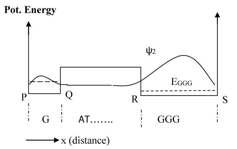
Figure 4: Wave function after the hole is inelastically scattered to the lowest energy level at EGGG. Other higher states will also have similar wave functions, but their probability of occupancy is much smaller than this lowest state.
This is the lower most state of the potential energy structure, and the backward transition to higher states by inelastic scattering has been ignored as the next higher state is about 0.5 eV higher than this lowest state, and has a very small probability of occupancy. Hence, the value of τ3 (time constant for hole transition to a higher state) is considered to be infinitely large in eqns. 10a-c. As before, α values are obtained by using eqn. 6d with j = 2. Hence, the total probability for product formation at each base site is given by
PG = PG0 + PG1 + PG2 (11)
PA = PA0 + PA1 + PA2 (12)
PGGG = PGGG0 + PGGG1 + PGGG2 (13)
In addition to giving the total amounts of products at G, A or GGG sites (eqns 11-13), this model also allows one to calculate product values within any specific location by taking into account the wavefunction distribution at that location. For example, we can calculate the distribution of products within the individual G locations of the GGG cluster. If GGG(1), GGG(2) (middle G) and GGG(3) are the three G locations within the GGG cluster (region RS as shown in figure 1), then the amounts of products formed at these individual locations are proportional to the ratio of the probability at that location (G) to the probability at the region encompassing the GGG cluster corresponding to each of the wave functions, ψ0, ψ1 and ψ2, and can be expressed as
(14)
where j = 0, 1 or 2 (corresponding to the subscripts of the wave functions ψ0, ψ1 and ψ2) and , where r is the G location within GGG (Figure 1) and assumes values 1,2 or 3 and . Since the calculation of α requires ψ0, ψ1, and ψ2 functions, in next section we discuss how to calculate these functions and their associated energies.
Applying QM model for calculating ψ0, ψ1, and ψ2
As mentioned above, these calculations were done numerically by using a method described in [30,31] and using the MATLAB series of programs [33]. In the calculation of ψ0 we assume that soon after the formation of the hole at G, it will not experience the potential due to GGG, for which we consider a potential profile with an infinitely extended A barriers to the right as shown in figure 2a. With the barrier height [22] of 0.73 eV, the lowest eigenstate for the G well (Figure 2a) has the energy of 0.64 eV. Then, we assume a potential structure like that shown in figure 2b and calculated the rate of tunneling through the barrier of A bases. After tunneling, the wave function is distributed as shown schematically in figure 3, and is represented by ψ1. Since tunneling is a coherent process both ψ0 and ψ1 will have the same energy (0.64 eV). Although ψ0 belongs to the lowest energy state for the potential structure of figure 2a, ψ1 does not for the potential structure of figure 3 or 4. The lowest eigenstate (ψ2) for the potential structure of figure 3 or 4 is substantially lower in energy with a value of 0.16 eV (EGGG). For this large energy gap, the possibility of back transfer of hole from the low energy GGG site to high energy G site has been neglected in our numerical calculation. Even though for illustration purposes we provided schematic diagrams of wavefunctions (Figures 2-4), some of the actual functions, as calculated from the potential structure are presented later (Figure 7a-c).
We also examined other immediately higher energy states (which ranges from 0.565 to 0.612 eV) for different barrier widths, and find that they contribute very little toward the hole population or product concentration due to their lower probability of occupancy, and hence, these excited states were ignored. It is important to know that the hole populations at different eigenstates are determined by the Maxwell Boltzmann probability distribution function.
Calculating current components for tunneling and inelastic scattering
In calculating tunneling and scattered current components, we first assumed Vi = 0 in the barrier region (but not in GGG) so that there is no inelastic scattering due to the barrier, and all the current that is observed at the boundary of G and (A)n is due to tunneling current (ST) only. Then, we introduced Vi in the barrier and calculated the current at G. This current includes both tunneling (ST) and inelastically scattered (SI) components. Thus, we separated the tunneling and scattered components from the total current and present results in table 1. Figure 5 shows how the ratio of tunneling to inelastic current density (ST/SI) decreases with an increased barrier width.
| Table 1:Tunneling and inelastic probability current components, ST, SI,their ratio, and time involved in hole decay from the lone G (τ2)base are presented for different barrier widths (n = 1- 16) of DNAbase sequence, G(A)nGGG. The S values are in units of number ofparticles (holes)/sec and time constants are in seconds. | ||||
| n | ST | SI | ST/SI | τ2 (sec) |
| 1 | 5.2E+06 | 8.0E+05 | 6.5E+00 | 5.6E-08 |
| 2 | 1.1E+05 | 2.5E+04 | 4.5E+00 | 2.4E-06 |
| 3 | 2.0E+04 | 2.0E+04 | 1.0E+00 | 9.8E-06 |
| 4 | 5.9E+03 | 2.6E+04 | 2.3E-01 | 1.4E-05 |
| 5 | 1.7E+03 | 2.9E+04 | 5.8E-02 | 1.6E-05 |
| 6 | 4.8E+02 | 3.1E+04 | 1.6E-02 | 1.6E-05 |
| 7 | 1.4E+02 | 3.1E+04 | 4.4E-03 | 1.6E-05 |
| 8 | 3.8E+01 | 3.1E+04 | 1.2E-03 | 1.6E-05 |
| 9 | 1.1E+01 | 3.1E+04 | 3.5E-04 | 1.6E-05 |
| 10 | 3.1E+00 | 3.1E+04 | 9.9E-05 | 1.6E-05 |
| 11 | 8.8E-01 | 3.1E+04 | 2.8E-05 | 1.6E-05 |
| 12 | 2.5E-01 | 3.1E+04 | 8.0E-06 | 1.6E-05 |
| 13 | 7.1E-02 | 3.1E+04 | 2.3E-06 | 1.6E-05 |
| 14 | 2.0E-02 | 3.1E+04 | 6.5E-07 | 1.6E-05 |
| 15 | 5.7E-03 | 3.1E+04 | 1.8E-07 | 1.6E-05 |
| 16 | 1.6E-03 | 3.1E+04 | 5.2E-08 | 1.6E-05 |
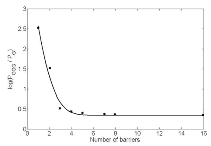
Figure 5: The tunneling (ST)/inelastic scattering (SI) ratios are presented against the number (n) of A barriers. The decrease in the ratio is most significant from n = 1-4, and then almost levels off. This result is obtained for the G(A)nGGG sequence with a potential energy barrier [22] of 0.73 eV.
Effective hole mass, imaginary potential and reaction time
Because of the lack of reported results on effective mass or imaginary potential in the literature, we obtained these values by fitting the experimental data [13] points. These parameters were needed for the predictions of oscillatory and non-oscillatory nature of the product yield. The best fit curve and the data points are shown in figure 6. The effective masses of the hole at the G (or GGG) and A sites are determined to be around 1.42 m0 and 1.50 m0 respectively, where m0 is the rest mass of an electron. These masses are in line with the typical hole masses that are considered in different charge transport phenomena in physics and electronic engineering. Similarly, the imaginary potential (Vi) value has been determined to be 0.25 × 10⁻¹⁰ eV.
Figure 6: Experimental data points [13] and theoretical solid curve are shown. The barriers are due to A bases lying in between the G base and the GGG base cluster.
As discussed above, in the process of hole transfer from G to GGG, if the hole remains at a particular base site longer than the time required for its reaction with water, products will form. For the water trapping reaction with a hole at the G site (forming G+), the experiment by Giese and Spichty [34] provides a rate constant (k) value of around 6.0 × 10⁴/s and hence, the time of reaction (τGC) of 1.67 × 10⁻⁵ sec (1/k). The same experiment also suggests reaction at the GGG site to be 3 times faster, and hence, τGGGC = τGC/3. While the experiment suggests a much slower reaction at the A site, no rate constant value has yet been reported for the water trapping reaction at this site. In the absence of such experimental data, we examined a number of values by considering rate at A to be 5, 10 or 15 times slower than that at the G site. These results suggest that 10 times slower rate or τAC = τGC × 10 gives a product concentration at A in better agreement with that of the experiment [13]. It is to be mentioned that only the percent product formation inside the barrier is dependent upon this value and has no effect on the overall findings of this study.
Nature of wave functions at different barrier widths
Figures 7a-c are representative hole probability functions (|ψ|2) for n = 1 and n = 6 of G(A)nGGG sequence obtained by applying the present QM model. The ψ0 function is presented in figure 7a and ψ1, and ψ2 are presented in figure 7b and 7c. As the barrier width is increased from n = 1 (Figure 7b) to n = 6 (Figure 7c), a remarkable change in ψ1 (dashed curve in 7b and 7c) function is noticed. As expected, for the smallest barrier width of n = 1, the wavefunction penetration within the barrier is significant suggesting relatively large hole concentrations at the A as well as GGG sites due to this wave function. For n > 4, the ψ1 function (see dashed curve, Figure 7c for n = 6) exhibits a much decreased penetration resulting in a negligibly small hole concentration within the distant A bases of the barrier and the GGG site, and thus, reaches a probability distribution that remains almost unchanged for larger n values (figures presented in supplemental information section).
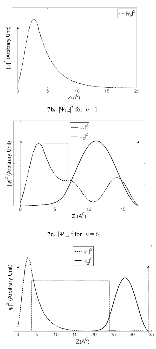
Figure 7: The probability functions, |ψ0|2, |ψ1,2|2 are presented against distance from the lone G base of the G(A)n_GGG sequence. Figure 7a represents |ψ0|2, and Figures 7b and 7c represent |ψ1,2|2 (dashed curve and solid curve) functions for n = 1 and n = 6 respectively. A substantial change in |ψ1|2 function with barrier width can be noticed from Figure 7b to 7c.
The ψ2 function (solid curve in 7b and 7c), on the other hand, shows large probability distributions at the G bases of the GGG cluster and much smaller probability distributions at the lone G base. Hence, ψ2 is primarily responsible for hole concentration at the GGG destination site. As the n value is increased from n = 1 to n = 6, the ψ2 function shows increased confinement in GGG site suggesting its major contribution toward product formation for larger n values. From the nature of these hole distribution functions it is obvious that the total hole concentrations at various base sites are given by the combined effect of ψ0, ψ1, and ψ2 functions.
Tunneling, inelastic scattering and CT mechanism
Figure 5 shows how the probability ratio of tunneling (ST) to scattering (SI) decreases when the barrier width is increased from n = 1-16. Our calculations suggest that the actual transition from ψ0 to ψ1 is a fast process (τ1 varies from 1.5 × 10⁻¹⁵ s for n = 1 to 1.2 × 10⁻¹⁸ s for n = 16) for which practically, there is no contribution from ψ0 towards the product formation. The major contribution of products comes from ψ1 and ψ2 states. The ratio of tunneling to inelastic scattering for ψ1 is about 6 for n = 1 (one intervening A base), which decreases sharply as n value is increased. Table 1 presents these values together with the time constant, τ2 (sec), for the decay of the wave function ψ1 from the lone G base. While the tunneling current, ST (number of holes/sec), decreases consistently with the increased n value, the inelastic scattering probability (SI) initially decreases upto n = 3, then increases slightly and finally levels off at around n = 5. A possible explanation for this trend can be due to the fact that the inelastic scattering is present both at A(n) as well as GGG sites. Eq.3 shows that the impact of imaginary potential will be stronger for smaller values of (E-V) or kinetic energy term while calculating the value of γ. Physically, movement of the hole in A(n) region will be a slower process compared to its movement in GGG as kinetic energy in GGG region is much higher. Hence, the effect of inelastic scattering would be stronger in A(n) and weaker in GGG region. For smaller values of n significant inelastic scattering takes place in GGG compared to A(n) as A(n) is still very thin and contain a very small fraction of the total wavefunction (Figure 7b). As n increases, wave function in GGG decreases quite rapidly but increases in A(n) gradually. So, the interplay of these two inelastic scattering effects make the overall inelastic scattering decrease as n increases from 1 to 3. After that (n = 4 and 5) the wavefunction in GGG becomes very small to have any significant impact but fraction of wavefunction in A(n) keeps on increasing very slowly which is apparent from the increase value of SI in table 1. For n > 5 the penetration of wavefunction inside A(n) saturates (Figure 7c) and the inelastic scattering does not show any further increase. Table 1 also shows that the decay time constant, τ2, increases with the increasing number of A bases until n = 4, and then remains constant. This result is consistent with the fact that a strong distance dependent CT takes place for n < 4 and a weak distance dependent CT takes place for n ≥ 4.
Product concentrations at different barrier widths
While hole concentrations at different base sites can be readily obtained from the probability wave functions (|ψ|2), and are related to the amount of product formed, the exact calculation of product concentration requires hole reactivity at a base site and the survival time of the hole. With these considerations, and the application of equations 5-13, the product concentrations have been calculated. Table 2 presents percent product concentrations at different base sites for G(A)nGGG system with n = 1-16. For the smallest barrier width of n = 1, a hole does not remain at the lone G or A site long enough to form any significant amount of products. Hence, the product concentration (P) is the largest at the GGG site (over 99%) and smallest at the lone G (0.27%) and A (0.15%) sites. As the barrier width is increased by adding another A base (n = 2), the hole finds it harder to get through the barrier, and hence, remains at the lone G and A sites for a longer amount of time. This results in larger product concentrations at the G and A sites of around 5% and 1%, respectively with the rest (94%) at the GGG site. This trend in concentration change is continued up to n = 4 when the product concentrations at the lone G, A and GGG sites are around 27%, 4% and 69% respectively. Interestingly, for n > 4, the product concentrations at the base sites remain almost unchanged. At these barrier widths (n > 4), tunneling is insignificant (Table 1) compared to inelastic scattering, and hence, CT is primarily due to inelastic scattering of the hole, which almost levels off at n > 4. It should be pointed out that although the tunneling effect is quite small at n > 4, it consistently decreases and may explain a very small decreasing trend in product formation with increased n values. Although cannot be noticed within our reported number of decimal places in table 2, this decrease in product formation reflects a longer hole transportation time from G to GGG when the number of intervening bases (n value) is increased.
| Table 2: Percent product (P) formation at different base sites of the G(A)nGGG sequence. A breakdown of PGGG into PGGG( 1), PGGG(2) and PGGG(3) corresponding to GGG(1), GGG(2) and GGG(3) (Figure 1) are also presented in the table. | |||||
| n | PG | PA | PGGG | ||
| PGGG(1) | PGGG(2) | PGGG(3) | |||
| 1 | 0.27 | 0.15 | 34.24 | 49.40 | 15.94 |
| 2 | 4.51 | 0.62 | 33.01 | 44.11 | 17.75 |
| 3 | 17.37 | 2.32 | 28.87 | 34.45 | 16.99 |
| 4 | 26.60 | 3.84 | 24.43 | 32.03 | 13.11 |
| 5 | 29.28 | 4.46 | 22.76 | 32.24 | 11.26 |
| 6 | 29.67 | 4.63 | 22.39 | 32.56 | 10.74 |
| 7 | 29.66 | 4.67 | 22.33 | 32.73 | 10.62 |
| 8 | 29.62 | 4.68 | 22.33 | 32.79 | 10.59 |
| 9 | 29.59 | 4.68 | 22.33 | 32.82 | 10.58 |
| 10 | 29.58 | 4.68 | 22.33 | 32.83 | 10.58 |
| 11 | 29.58 | 4.68 | 22.33 | 32.83 | 10.58 |
| 12 | 29.58 | 4.68 | 22.33 | 32.83 | 10.58 |
| 13 | 29.58 | 4.68 | 22.33 | 32.83 | 10.58 |
| 14 | 29.58 | 4.68 | 22.33 | 32.83 | 10.58 |
| 15 | 29.58 | 4.68 | 22.33 | 32.83 | 10.58 |
| 16 | 29.58 | 4.68 | 22.33 | 32.83 | 10.58 |
As mentioned earlier, our QM model gives product concentrations not only at the G, A and GGG sites it also predicts product concentrations at the individual base site of the GGG base cluster (Figure 1). For each n value, the product concentration, as calculated by using eq.14, is largest at the middle G (GGG(2), Table 2) and smallest at the farthest G (GGG(3), Table 2) of the GGG cluster, and is in agreement with the experimental results [13].
Hopping vs. other inelastic scattering mechanisms of CT
In our QM model, the imaginary potential incorporates a loss mechanism of the hole from any particular region. Hopping through the bridge is one such mechanism in which the hole acquires enough energy to overcome the barrier, and hence, leaves its original energy state to land onto the next state. In addition, there are other inelastic processes like chemical reactions that may also cause hole loss from a particular region. So, it is quite possible that more than one inelastic process may take place in a region. For example, within the bridge region the hole loss can be due to both hopping as well as chemical reactions. If the time constants for these individual processes are known, one would be able to estimate the extent of hopping through the bridge.
Origin of oscillatory/non-oscillatory CT yield
In order to examine the oscillatory CT yield in Barton’s experiment that involves Ap*(A)nG sequence, and non-oscillatory CT yield in Giese’s experiment for G(A)nGGG sequence, following calculations were carried out. First, we calculated the energy barrier for the Ap(A)nG sequence by using the same procedure as was used for G(A)nGGG sequence [26]. In brief, reorganization energies (λ) were calculated by using the B3LYP/6-311++G** method [35-38] followed by the application of following Marcus’ eqn.(eqn. 15) [39]:
(15)
These calculations yield a barrier height (Ea) of 0.19 ev, which is significantly smaller than that of G(A)nGGG system [26] with a barrier height of 0.73 ev. In eqn (15) ∆G is the free energy change for hole transfer from the donor to the acceptor.
In Giese’s system we obtained a bound state with an energy value of 0.64 ev, as discussed earlier, and is lower than the barrier height (0.73 ev) [26]. The same method, when applied to Barton’s system, did not result in any bound energy state suggesting that the energy of the hole for Ap*(A)nG system is larger than the barrier height (0.19 ev). These two distinct differences, E < Vo for Giese’s system, and E > Vo for Barton’s system provide incentive to apply QM transmission expressions (T, eqns 16 and 17) to see how the probability of hole transmission change in these two situations. Eqns 16 and 17 are well-known QM expressions derived for a rectangular barrier (like ours, without the potential wall on far left or far right of figure 1) with width a. For hole energy less than the barrier height, E < Vo, there is a non-zero transmission probability (tunneling) given by eqn 16, and is presented in figure 8a for different K1a (or a) values. In eqns 16 and 17, t is the amplitude of transmitted wave, T is the probability of transmission (or transmission coefficient), a is the barrier width, and k1 is a constant for a particular hole energy.
(16)
For energies greater than the barrier height, E > Vo, the T value is given by eqn 17 and is presented in figure 8b.
(17)
For eqn 16 we used Vo = 0.73 ev, E = 0.64 ev, and for eqn 17 we used Vo = 0.19 ev, and selected an E value larger than the barrier height with a value of 0.43 ev. Although 0.43 ev energy value has been selected arbitrarily, the value represents an approximate energy that is given off when a hole transfers from Ap+ to a G base involving ionization energy (IE) of G (to form G+) and electron affinity of Ap+ (-IE of Ap). The IE values were calculated by applying the B3LYP/6-311++G** method.
Since figure 8a represents only the tunneling effect, there is no flat weak distance dependence segment of the curve as in figurer 6. This confirms our finding that a second mechanism (inelastic scattering) must be present to account for the weak distance dependence of CT yield when E < Vo. The oscillatory nature of hole transmission is indeed observed for E > Vo (Figure 8b), which represents Barton’s experimental condition. Classically, the condition E > Vo would mean that the hole will be transferred from the donor to acceptor by simply passing over the barrier resulting in 100% transmission. However, in quantum mechanics, the incident wave from the donor side will suffer reflection at each of the potential discontinuities of the barrier even if E > Vo. Under such a condition, change in bridge length will change the phase of the forward and the reflected propagating waves and their interference give rise to the oscillations as observed in the transmission co-efficient shown in figure 8b. It is expected that the product formation at different base sites will be related to the hole transmission probability from a donor to the acceptor. It is interesting to note that the period of oscillation is around 3.0 (in K1a unit) in figure 8b, which corresponds to a barrier thickness (a) of 10.1 Å with 4 intervening A bases (10.1/3.4 + 1). For this calculation, first k1 value (2.98 × 10⁹ m-1) was obtained assuming the mass of the hole to be close to (1.4 m0) that obtained for a G or an A base in G(A)nGGG system (discussed earlier). The number of intervening A bases, thus obtained, is very close to that of the experiment with a value of around 3 (ref 8). Although the period of oscillation in figure 8b is close to that obtained in experiment, unlike the experiment, the oscillatory function does not decrease with the increased barrier thickness (a). This is presumably the result of the simplicity of the transmission analysis in which back electron or hole (BET) transfer resulting from the hole reflection from the potential wall on the far right (Figure 1) has been ignored. In spite of this simplicity, the transmission analysis provides the origin of oscillatory/non-oscillatory patterns in CT yield and explains both Barton’s and Giese’s result. A more rigorous study is now underway to explain quantitatively the decreasing oscillatory function of the CT yield when the barrier width is increased.
Comparison with density matrix theory
May and Schreiber [40] in their density matrix theory (DMT) consider LUMOs (lowest unoccupied molecular orbitals) to be the localization centers for the extra electron from the donor. This extra electron moves within the pseudo-potential of the total electronic system of the entire molecule. In addition, the Hamiltonian, as defined in the DMT, also includes potential energy terms corresponding to contributions from environment (solvent) as well as molecular vibrations. For a large molecular system like G(A)nGGG such calculations become very complicated. In our study much simpler treatment has been followed in which a hole moves within a rectangular potential barrier of A bases. Instead of LUMOs we considered bound states defined by a G base and the barrier due to A bases. Unlike DMT, the solvent effect has only been considered in an indirect manner through the use of an effective hole mass as well as the reaction rate (time constant) obtained by fitting the experimental data. Similarly, the effect of vibration on hole transfer has also been considered via the use of the imaginary potential.
In our model simultaneous interplay of two mechanisms, tunneling and inelastic scattering, have been considered to explain the experimental results [13]. For E > Vo (Giese’s experimental condition), the ratio of tunneling to inelastic scattering current decreases sharply from a value of around 6 for n = 1 to around 0.06 for n = 5. Without considering any mechanism change in advance for n > 3 or without explicitly considering hole hopping from one A to another, the model explains experimental results of product formations at different base sites. At every n value both tunneling and inelastic scattering takes place as the hole migrates from G to GGG. As in experiment, the present model explains a strong distance dependence of CT for n = 1-3 and a weak distance dependence for n > 3 (Figure 6). While most models consider the onset of a distance independent A-hopping mechanism for n > 3, our model predicts dominance of distance independent inelastic scattering (SI) after an initial drop from n = 1 to n = 3 (Table 1). The weak to very weak distance dependence for n > 3 is due to a decreasing tunneling (ST) probability superimposed on to the inelastic scattering values. For E > Vo an oscillatory function is obtained with a period of oscillation close to that obtained in the experiment.
The authors acknowledge helpful discussions with Joseph Genereux of Professor Barton’s group, and computation time provided on Linux machines by Numerically Intensive Computing Group at the center for Academic Computing at Penn State for some of the calculations.
1. Burrows CJ, Muller JG. Oxidative Nucleobase Modifications Leading to Strand Scission. Chem Rev. 1998; 98: 1109-1152. PubMed: https://www.ncbi.nlm.nih.gov/pubmed/11848927
2. Eley DD, Spivey DI. Semiconductivity of organic substances. Trans Faraday Soc. 1962; 58: 411-415.
3. Braun E, Eichen Y, Sivan U, Ben-Yoseph G. DNA-templated assembly and electrode attachment of a conducting silver wire. Nature. 1998; 391: 775-778. PubMed: https://www.ncbi.nlm.nih.gov/pubmed/9486645
4. Braun E, Eichen Y, Sivan U, Ben-Yoseph G. DNA-templated assembly and electrode attachment of a conducting silver wire. Nature. 1998; 391: 775-778. PubMed: https://www.ncbi.nlm.nih.gov/pubmed/9486645
5. Nitzan A, Ratner MA. Electron transport in molecular wire junctions. Science. 2003; 300: 1384-1389. PubMed: https://www.ncbi.nlm.nih.gov/pubmed/12775831
6. Kasumov AY, Kociak M, Guéron S, Reulet B, Volkov VT, et al. Proximity-induced superconductivity in DNA. Science. 2001; 291: 280-282. PubMed: https://www.ncbi.nlm.nih.gov/pubmed/11209072
7. Khan A. Substituent group effects on reorganization and activation energies; Theoretical study of charge transfer reaction through DNA. Chem Phys Lett. 2010; 486: 154–159.
8. O’Neill MA, Barton JK. DNA charge transport: conformationally gated hopping through stacked domains. J Am Chem Soc. 2004; 126: 11471-11483.
9. O’Neill MA, Barton JK. DNA-Mediated Charge Transport Requires Conformational Motion of the DNA Bases: Elimination of Charge Transport in Rigid Glasses at 77 K. J Am Chem Soc. 2004; 126: 13234-13235.
10. (a) Delaney S, Barton JK. Long-range DNA charge transport. Org Chem. 2003; 68: 6475-6483. PubMed: https://www.ncbi.nlm.nih.gov/pubmed/12919006
b) Yoo J, Delaney S, Stemp ED, Barton JK. Rapid radical formation by DNA charge transport through sequences lacking intervening guanines. J Am Chem Soc. 2003; 125: 6640-6641. PubMed: https://www.ncbi.nlm.nih.gov/pubmed/12769567
(c) O'Neill MA, Barton JK. 2-Aminopurine: a probe of structural dynamics and charge transfer in DNA and DNA: RNA hybrids. J Am Chem Soc. 2002; 124: 13053-13066. PubMed: https://www.ncbi.nlm.nih.gov/pubmed/12405832
(d) Wan C, Fiebig T, Schiemann O, Barton JK, Zewail AH. Femtosecond direct observation of charge transfer between bases in DNA. Proc. Natl Acad Sci USA. 2000; 97: 14052-14055. PubMed: https://www.ncbi.nlm.nih.gov/pubmed/11106376
(e) Wan C, Fiebig T, Kelley SO, Treadway CR, Barton JK, et al. Femtosecond dynamics of DNA-mediated electron transfer. Proc Natl Acad Sci USA. 1999; 96: 6014-6019. PubMed: https://www.ncbi.nlm.nih.gov/pmc/articles/PMC26827/
(f) Kelley SO, Barton JK. Electron transfer between bases in double helical DNA. Science. 1999; 283: 375-381. PubMed: https://www.ncbi.nlm.nih.gov/pubmed/9888851
(g) Turro NJ, Barton JK. Paradigms, supermolecules, electron transfer and chemistry at a distance. What’s the problem? The science or paradigm? J Biol Inorg Chem. 1998; 3: 201-209.
11. (a) Lewis FD, Liu JQ, Weigel W, Rettig W, Kurnikov IV, et al. Donor-bridge-acceptor energetics determines the distance dependence of electron tunneling in DNA. Proc Natl Acad Sci USA. 2002; 99: 12536 - 12541.
(b) Lewis FD, Liu X, Miller SE, Hayes RT, Wasielewski MR. Formation and Decay of Localized Contract Radical Ion Pairs in DNA Hairpins. J Am Chem Soc. 2002; 124: 14020-14026. PubMed: https://www.ncbi.nlm.nih.gov/pubmed/12440900
12. Meggers E, Michel-Beyerle ME, Giese B. Sequence dependent long-range hold transport in DNA. J. Am. Chem. Soc. 1998; 120: 12950-12955.
13. Giese B, Amaudrut J, Köhler AK, Spormann M, Wessely S. Direct observation of hole transfer through DNA by hopping between adenine bases and by tunneling. Nature. 2001; 412: 318-320. https://www.ncbi.nlm.nih.gov/pubmed/11460159
14. Ly D, Sanii L, Schuster GB. Mechanism of charge transport in DNA: internally-linked anthraquinone conjugates support phonon-assisted polaron hopping. J Am Chem Soc. 1999; 121: 9400-9410.
15. Paul A, Watson RM, Wierzbinski E, Davis KL, Sha A, et al. Distance Dependence of the Charge Transfer Rate for Peptide Nucleic Acid Monolayers. J Phys Chem B. 2010; 114: 14140-14148. PubMed: https://www.ncbi.nlm.nih.gov/pubmed/19691305
16. (a) Jortner J, Bixon M, Voityuk AA, Rosch J. Superexchange mediated charge hopping in DNA. Phys Chem A. 2002; 106: 7599-7606.
(b) Bixon M, Jortner J. Long-range and very long-range charge transport in DNA. Chem Phys. 2002; 281: 393-408.
(c) Bixon M, Jortner J. Hole trapping, detrapping and hopping in DNA. Phys Chem A. 2001; 105: 10322-10328.
(d) Bixon M, Jortner J. Charge transport in DNA via thermally induced hopping. Am Chem Soc. 2001; 123: 12556-12567. PubMed: https://www.ncbi.nlm.nih.gov/pubmed/11741420
(e) Bixon M, Jortner J. Energetic control and kinetics of hole migration in DNA. J Phys Chem B. 2000; 104: 3906-3913;
(f) Bixon M, Giese B, Wessely S, Langenbacher T, Michel-Beyerle ME, et al. Long-range charge hopping in DNA. Proc Natl Acad Sci USA. 1999; 96: 11713-11716. PubMed: https://www.ncbi.nlm.nih.gov/pubmed/10518515
(g) Jortner J, Bixon M, Langenbacher T, Michel-Beyerle ME. Charge transfer and transport in DNA. Proc. Natl. Acad. Sci. USA. 1998; 95: 12759-12765.
17. (a) Berlin YA, Burin AL, Ratner MA. Elementary steps for charge transport in DNA: thermal activation vs. tunneling. Physica. 2002; 275: 61-74.
(b) Berlin YA, Burin AL, Ratner MA. Charge hopping in DNA. J Am Chem Soc. 2001; 123: 2: 260-268. PubMed: https://www.ncbi.nlm.nih.gov/pubmed/11456512
(c) Berlin YA, Burin AL, Ratner MA. On the long-range charge transfer in DNA. J Phys Chem A. 2000; 104; 443-445.
(d) Grozema FC, Berlin YA, Siebbeles LDA. Mechanism of Charge Migration through DNA: Molecular Wire Behavior, Single-Step Tunneling or Hopping. J Am Chem Soc. 2000; 122: 10903-10909.
18. Tong GSM, Kurnikov IV, Beratan DN. Tunneling energy effects on GC oxidation in DNA. J Phys Chem B. 2002; 106: 2381-2392.
19. (a) Li XQ, Zhang HY, Yan YJ. A superexchange-mediated sequential hopping theory for charge transfer in DNA. J Phys Chem A. 2001; 105: 9563-9567.
(b) Zhang HY, Li XQ, Han P, Yu XY, Yan YJ. A partially incoherent rate theory of long-range charge transfer in deoxyribose nucleic acid. J Chem Phys. 2002; 117: 4578.
20. Renger T, Marcus RA. Variable-range hopping electron transfer through disordered bridge states: Application to DNA. J Phys Chem A. 2003; 107: 8404-8419.
21. (a) Conwell EM. Polarons and Transport in DNA. Top Curr Chem. 2004; 237: 73-102.
(b) Conwell EM. Charge transport in DNA in solution: The role of polarons. Proc Natl Acad Sci USA. 2005; 102: 8795-8799.
22. Hatcher E, Balaeff A, Keinan S, Venkatramani R, Beratan DN. PNA versus DNA: Effects of Structural Fluctuations on Electronic Structure and Hole-Transport Mechanisms. J Am Chem Soc. 2008; 130: 11752-11761.
23. Genereux JC, Barton JK. Mechanisms for DNA charge transport. Chem Rev. 2010; 110: 1642–1662. PubMed: https://www.ncbi.nlm.nih.gov/pmc/articles/PMC2879062/
24. Adhikary A, Kumar A, Khanduri D, Sevilla MD. Effect of Base Stacking on the Acid-Base Properties of the Adenine Cation Radical in Solution: ESR and DFT Studies. J. Am. Chem. Soc. 2008; 130: 10282–10292.
25. Ptasińska S1, Denifl S, Scheier P, Märk TD. Inelastic electron interaction (attachment/ionization) with deoxyribose. J Chem Phys. 2004; 120: 8505. PubMed: https://www.ncbi.nlm.nih.gov/pubmed/15267776
26. Khan A. Reorganization and activation energies for hole transfer processes in DNA: a theoretical study. J Chem Phys. 2008; 128: 075101-6. PubMed: https://www.ncbi.nlm.nih.gov/pubmed/18298173
27. Senthilkumar K, Grozema FC, Guerra CF, Bickelhaupt FM, Lewis FD, et al. Absolute Rates of Hole Transfer in DNA. J. Am. Chem. Soc. 2005; 127: 14894-14903. PubMed: https://www.ncbi.nlm.nih.gov/pubmed/16231945
28. Yildiz A, Kasap M. The temperature dependence of the inelastic scattering time in InGaN grown by MOVPE. Low temp. Phys. 2010; 36: 320.
29. Santhanam BP, Prober DE. Inelastic electron scattering mechanisms in clean aluminum films. Phys Rev B. 1984; 29: 3733.
30. Khondker AN, Khan MR, Anwar AFM. Transmission line analogy of resonance tunneling phenomena: The generalized impendance concept. J. Appl. Phys. 1988; 63: 5191.
31. Haque A, Khondker AN. An efficient technique to calculate the normalized wave functions in arbitrary one-dimensional quantum well structures. J Appl Phys. 1998; 84: 5802.
32. Khan A. Effect of guanine-cytosine base pair orientation and cluster size on ionization energy and charge distribution: A theoretical study. Computational & Theoretical Chemistry. 2014; 1047: 67-70.
33. MATLAB, The Math Works, Inc. 3 Apple Hill Drive, Natick, MA 01760-2098, USA.
34. Giese B, Spichty M. Long distance charge transport through DNA: Quantification and extension of the hopping model. Chem Phys Chem. 2000; 1: 195-198.
35. Becke AD. Density-functional exchange-energy approximation with correct asymptotic behavior. Phys. Rev. A 1988; 38: 3098-3100. PubMed: https://www.ncbi.nlm.nih.gov/pubmed/9900728
36. Becke AD. Density-functional thermochemistry. III. The role of exact exchange. J Chem Phys. 1993; 98: 5648-5652.
37. Lee C, Yang W, Parr RG. Development of the Colle-Salvetti conelation energy formula into a functional of the electron densitya. Phys Rev B. 1988; 37: 785-789. PubMed: https://www.ncbi.nlm.nih.gov/pubmed/9944570
38. Vosko SH, Wilk L, Nusair M. Accurate spin-dependent electron liquid correlation energies for local spin density calculations: a critical analysis. Can J Phys. 1980; 58: 1200-1211.
39. (a) Marcus RA, Sutin N. Electron transfers in chemistry and biology. Biochim Biophys Acta. 1985; 811: 265-322.
(b) Bolton LB, Archer MD. Basic Electron-Transfer Theory In ET in Inorganic, Organic & Biological Systems, Advances in Chemistry Series. 1991; 220: 7-23.