
More Information
Submitted: July 31, 2023 | Approved: August 16, 2023 | Published: August 17, 2023
How to cite this article: Walia S. Investigating Thermal Conductivity of Ferrofluids. Int J Phys Res Appl. 2023; 6: 144-153.
DOI: 10.29328/journal.ijpra.1001064
Copyright License: © 2023 Walia S. This is an open access article distributed under the Creative Commons Attribution License, which permits unrestricted use, distribution, and reproduction in any medium, provided the original work is properly cited.
Keywords: Nanofluids; Ferrofluids; Thermal conductivity; Heat transfer; Brownian motion

Investigating Thermal Conductivity of Ferrofluids
Sumeir Walia*
Dhirubhai Ambani International School, Mumbai, India
*Address for Correspondence: Sumeir Walia, Dhirubhai Ambani International School, Mumbai, India, Email: [email protected]
Heat transfer is one of the most important aspects of large-scale industries and machines, linking importantly to the efficiency associated with different mechanisms while also emphasizing the importance of sustainable, low-cost methods of heat transfer. One such method is the use of ferrofluids. Through this paper, it is clearly explained that the conductivity of ferrofluids has vast applications across industries and using its magnetic and thermal properties, it can be a cost-effective solution as well. Previously researched works in this field ferrofluids are also acknowledged and furthered as per experimental data.
Nanotechnology is the fastest-growing area of modern research due to its broad-spectrum applications: medicine, automobiles, etc. Irrespective of the size or type of industry, a common requirement to all is an efficient heat-transfer mechanism. Cooling of heavy machinery maintains operational functionality and longevity.
Conventionally coolants like water flow through pipes around heated machinery. Nanofluids have emerged as potential replacements in such cooling systems. Their versatile properties allow for the manipulation of heat transfer through them.
They possess greater heat-transfer ability and are efficient in small quantities–vital to cooling of microprocessors and Micro-Electro-Mechanical Systems (MEMS) [1].
To explore one such methodology used to enhance the heat transfer capabilities of specific Nanofluids, the following research question was derived:
How is the thermal conductivity of a model (50 𝝁m – 100 𝝁m) Ferrofluid (Fe2O3), contained in a glass test tube of length 0.15 m and diameter 0.036 m and placed axially within 50-turn and 200-turn solenoids, affected when an increasing voltage (0V to 4.5V) increases the magnetic field strength (0.023 mT to 0.310 mT) across the solenoid?
Nanofluids can be characterized as nanoparticles of substances like metal or metallic- oxides dispersed in the base fluid. Ferrofluids (also referred to as Magnetic Nanofluids or MNFs) are colloidal solutions containing super-paramagnetic particles [2,3] in a non-magnetic base. Ferrofluids thus demonstrate both magnetic characteristics and fluid properties. Base fluids can be organic or inorganic, however, with regard to heat-transfer properties, fluids with relatively higher conductivity and heat capacity are preferred like water and oils. The magnetic particles can be ferromagnetic in nature which includes metals like iron and cobalt, or even metallic oxides like Fe2O3 or Al2O3.
Thermal Conductivity is a characteristic property of any material. A higher thermal conductivity represents a higher heat-transfer rate. In Nanofluids, thermal conduction takes place through microscopic collisions of nanoparticles with each other and molecules of base fluid.
Originally, it was considered that adding nanoparticles of higher thermal conductivity to an industrially used coolant like water would greatly enhance the thermal conductivity, culminating in volumes of research using TiO2, Cu, and Ag. However, Honk TJ and Choi CJ [4] proved through their investigations that solid materials with higher conductivities weren’t always effective. This, along with the idea of controlling the thermal conductivity of fluid cooling systems such that a “reversible switchable thermal fluid” be created, ushered in a great deal of research into the enhancement of thermal conductivity of nanofluids using external magnetic fields.
Works of scientists like Krichler [5] and Li Q. Xuan Y [6] have demonstrated the impact an external magnetic field has on nanofluids. To understand these effects, it’s necessary to understand the theoretical methods of heat transfer in such fluids.
a) Brownian motion is the term given to random movements of molecules and particles in fluids, i.e. liquids and gases, at a finite temperature [7]. Inelastic collisions with molecules of base fluid cause nanoparticles to undergo “zig-zag” movement. In regard to heat transfer, Brownian- motion theory suggests that when heat energy is to be transferred, the particles closer to the heat-source gain kinetic energy, thereby causing intense movement. Under these conditions, nanoparticles can transfer this heat energy by:They diffuse through fluid towards the cooler end where they collide with surrounding particles and increase their kinetic energy, leading to temperature rise.
b) Creating micro-convection of base liquid molecules which transfers heat from the region of the energized nanoparticles to the cooler region.
These effects were considered to enhance the thermal conductivity of fluid as there would be an efficient convectional mechanism between nanoparticles and fluid molecules [8].
Scientists like Li Q, Xuan Y and Philip J [9] further investi-gated the impact of volume fraction [10] of nanoparticles. Volume fraction refers to the ratio of the volume of constituents added to the volume of the entire solution after mixing. Their investigations demonstrated that decreasing particle sizes enhanced thermal conductivity but only till a certain limit.
Brownian-motion theory would be favored by decreasing particle sizes due to more particles and greater surface area for heat transfer (Figure 1). But these studies showed that Brownian motion accounted for only a certain amount of enhancement. This led to the NanoParticle Clustering Model.
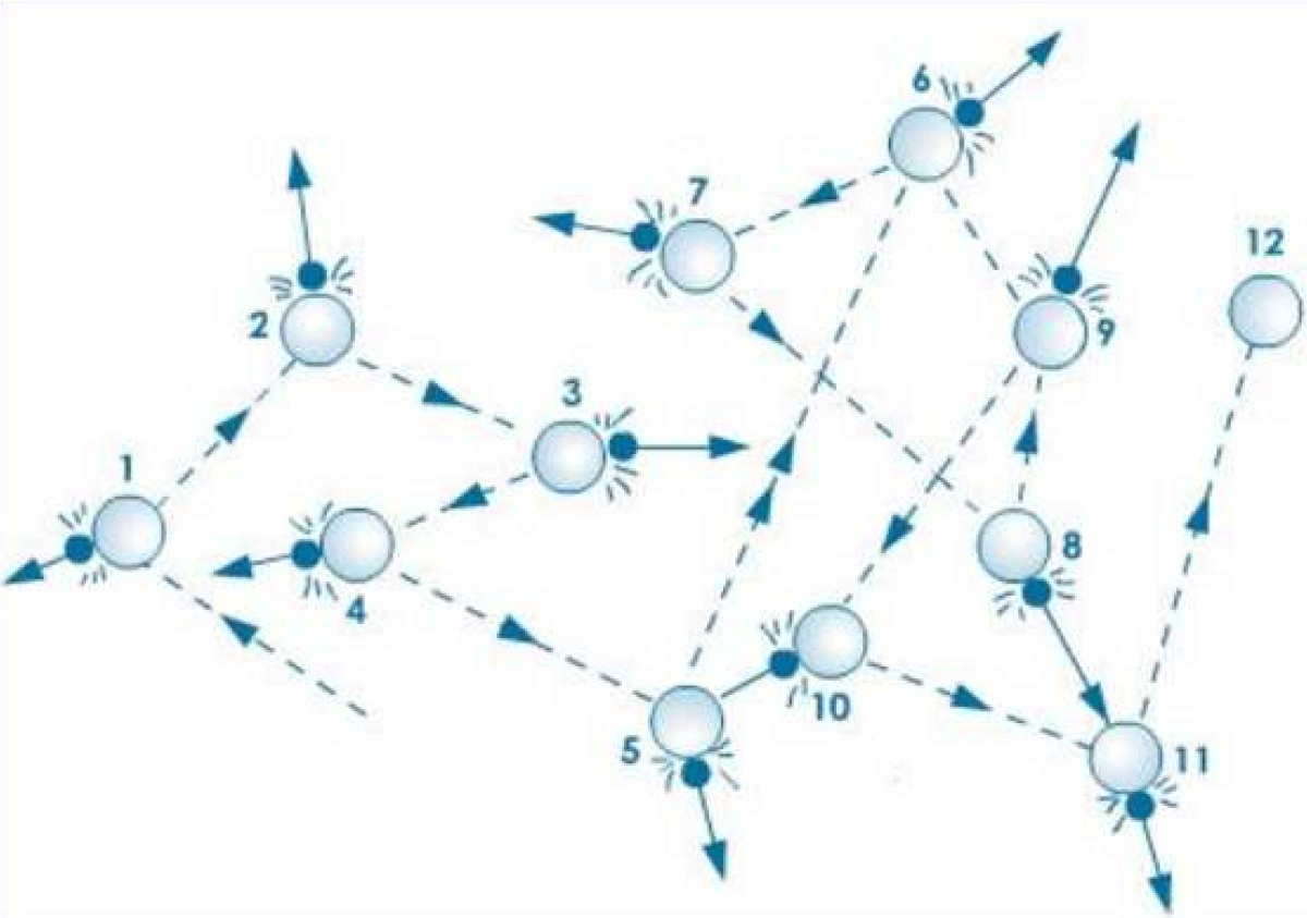
Figure 1: Random Movement of Particles and molecules in Brownian Motion [28].
Perhaps the most widely-acclaimed model for heat transfer in Nanofluids. In colloidal systems, suspended particles are almost evenly distributed in fluids. Nano-particle clustering model works on the aggregate formations of such distributed particles [11].
Aggregation of nanoparticles into isolated clusters, or ideally into long, linear chains is proposed as the main mechanism behind improved thermal conductivity of Nanofluids over industrial coolants as seen in Figure 2.
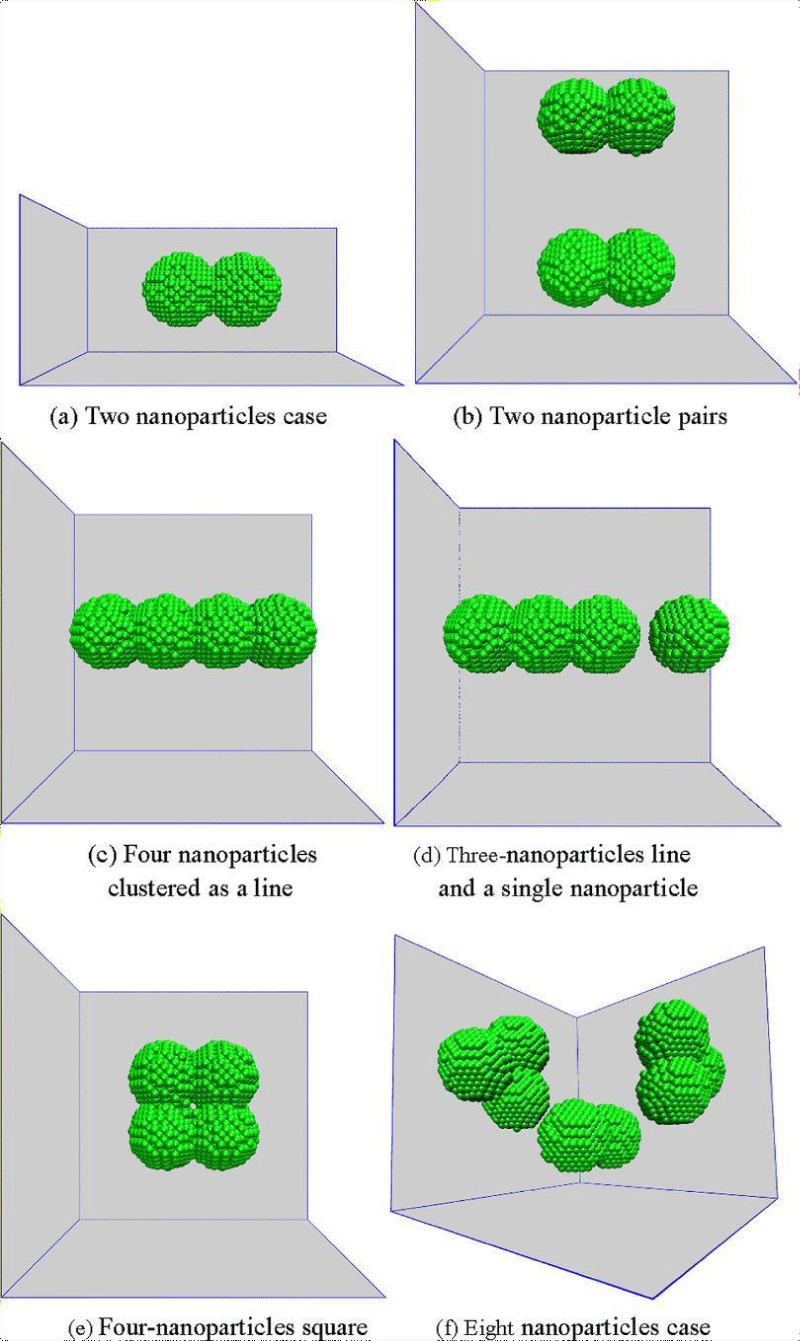
Figure 2: Types of Aggregate Cluster Nanoparticles tend to form [29].
These aggregations form long and highly conductive nanoparticle chains, which are particles of high thermal conductivity themselves, which perform as pathways for heat transfer, causing faster, efficient heat flow over long distances.
Aggregates form due to the superparamagnetic nature of nanoparticles. ‘Superparamagnetic nature’ refers to when particles can form weak, self-induced magnetic fields and can instantly switch their magnetism based on temperature-gradient around [12].
Under such conditions, nanoparticles cling due to magnetic attraction and form structures like chains, rings, or two-dimensional, three-dimensional lattice structures [13].
Without these aggregations, the distribution morphology of nanoparticles is disordered and the thermal conductivity is isotropic-even in all directions. However, in these micro-structures, thermal conductivity becomes anisotropic (unidirectional). Scientists like Zhu H and Jiang W conducted investigations into the Nanoparticle clustering model and concluded positively that clusters significantly enhanced thermal conductivity.
Figure 3 demonstrates these aggregates. Clearly observable that in (a), the particles are dispersed and widespread, however in (b), they cluster together forming connected, chain-like bridge structures.
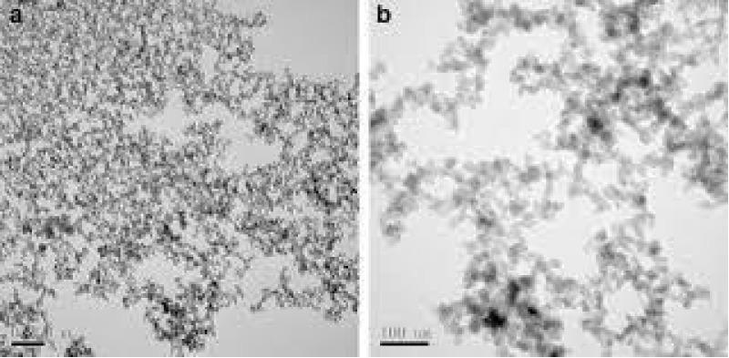
Figure 3: Aggregation Mechanism [14].
This behavior of nanoparticles stimulated studies into the effects of external magnetic- fields applied on Nanofluids. It was experimentally proven that external magnetic fields had powerful effects on micro-structure formations, engendering thermal conductivity enhancement in Nanofluids. These effects were guided by the intensity and orientation of the field.
Experiments were conducted with magnetic fields applied perpendicularly and parallel to the desired direction of heat flow (along temperature gradient) [15]. Magnetic fields applied perpendicularly negligible effects on the thermal conductivity of Nanofluid, irrespective of magnitude. However, when external magnetic fields were applied parallel to the temperature- gradient, the thermal conductivity of the Nanofluid greatly increased. Stronger magnetic fields increased heat conduction. Linking to the nanoparticle clustering model, where due to stronger fields, nanoparticles had reduced inter-particle distance and formed compact chains as shown in Figure 4. It was concluded that when the magnetic field was parallel to the temperature gradient, the aggregate- structures formed were more efficient in ensuring antistrophic thermal conductivity.
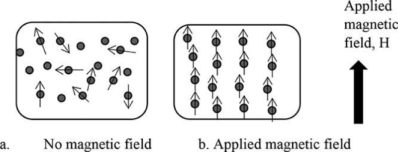
Figure 4: of external Magnetic Field on Nanoparticles [24].
Model-ferrofluid synthesis – Fe2O3
The model-Ferrofluid used was a mixture of powdered-Haematite (Fe2O3) and carrier-fluid water. Generally, Nanofluids are categorized into two types of mixture models based on physical Properties-Single Phase model and Two-Phase model. In the Single Phase model, the fluid is considered to be a homogenous mixture while the Two-Phase (or Mixture) model considers the nanoparticles merely suspended in carrier fluid.
The synthesized fluid is a Two-Phase mixture with a particle size of Fe2O3-powder ranging from 50 𝝁m – 100 𝝁m, greater than nano-scale and hence, model-Ferrofluid:
One assumption made while modelling the Ferrofluid was that the particle size is large enough to prevent the ‘clumping’ of particles. In an actual Nanofluid, clumping of particles due to extremely strong external magnetic fields may alter the shape of the chain or cause a “zippering” effect, which would result in broken micro-structures and the thermal conductivity wouldn’t increase. This also occurs because of weak Van der Waal’s forces present between molecules along with temporary magnetic dipole that is created due to its superparamagnetic nature. But because these particles aren’t of the nano-scale, it would be unlikely for magnetic-field strength to be large enough to cause clumping.
Carrier-fluid-water
Investigations prove that thermal conductivity enhancement is the greatest in carrier fluids with low thermal conductivities themselves. However, absolute thermal conductivity is higher for Nanofluids having base fluid with high thermal conductivity [16]. Considering this, water qualified as easily-available and best-suited. Distilled water was used to ensure that impurities weren’t present which could bring about added conduction or affect the magnetic- field.
Nano particle-haematite
Haematite was used due to the relatively high thermal conductivity of iron and its oxides. Haematite and magnetite are frequently used in Nanofluids and studies have investigated their functionality.
Though low volume fraction improved thermal conductivity, because nanoparticles are being modelled, a relatively higher fraction would be ideal. 20 g of Fe2O3 was mixed in 40 ml of distilled water for an overall volume of 60 ml. Volume fraction (volume percent) is therefore 33.33%. This adds a sufficient amount of solute that won’t settle down completely.
(1)
a) The Setup/ProceduTwo Solenoids: The experiment used two solenoids of varying lengths and turn numbers. Test tubes containing Ferrofluids are inserted into hollow tubular regions, along the axis of the solenoid, parallel to the direction of the magnetic field inside (Figure 5A). The horizontal orientation of tubes inside the solenoid allows the metallic particles (heavier than nanoparticles) to spread out. It minimizes gravitational effects on these particles which could impact the thermal conduction due to vertical movement. The glass test tubes are poor conductors of heat, further ensuring no heat is lost during the process.
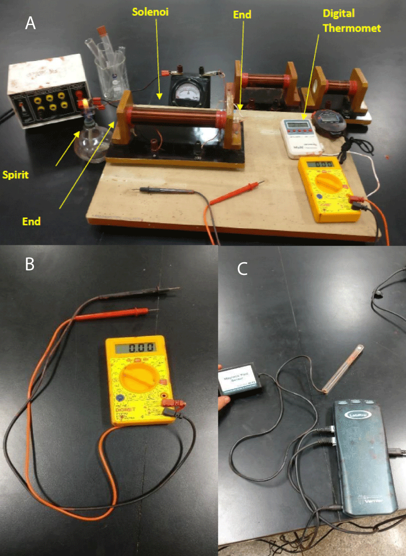
Figure 5: Experimental Setup. B: Multimeter. C: Magnetic Probe.
However, test-tube walls are extremely thin and could lead to radial heat loss by conduction. Initially, it was planned that test tubes be wrapped in insulators like wool but this wasn’t done because the thick, insulating layer could cause hindrance between the weak magnetic field generated by the solenoid and the fluid, resulting in lower temperatures measured at End-B.
Length (L), number of turns (N), and calculated turn density (n) of each solenoid is given in Table 1. The turn density is directly proportional to magnetic-field strength:
| >Table 1: Length of each solenoid. | ||
| >Number of Turns (N) | >Length (L ± 0.000 5/m) | >Turn Density (n ± N/m) |
| >50 | >0.09 | >555.56 ± 3.09 |
| >200 | >0.19 | >1052.63 ± 2.77 |
B = 𝜇0𝑛𝐼 [17] (2)
B = Magnetic-field strength
N = Turn density
Magnetic constant 𝜇0 = permeability of free space (4𝜋 × 10-7 T amp-1 m-1)
I = current in solenoid-coils.
The turn density: (3)b) Power Supply/Ammeter/Multimeter/Magnetic-Probe: A power supply applies the voltage measured by the multimeter (Figure 5B) across the solenoid. An ammeter measures the current (I) and a magnetic probe (Figure 5C) measures the magnetic field inside the solenoid using Logger-Pro software. The magnetic field across the solenoid was measured in microteslas (mT) (Tables 2,3). The earth’s magnetic field itself is roughly 25 - 65 microteslas (at the surface). However, this external magnetic field has minimum impact on solenoids. Given the dimensions of the test tube and quantity of fluid, it is predicted that the given range will sufficiently influence the ferrofluid. From Figure 6, there is a significant increase in magnetic-probe reading after voltage is applied as compared to earth’s field alone, indicated as 0.02mT before the application of voltage. The relationship is not linear and the slope gradually decreases. There are large decreases in slope for both solenoids between the second and third multimeter readings. Using current readings of the Ammeter, theoretical magnetic field strength can be calculated using
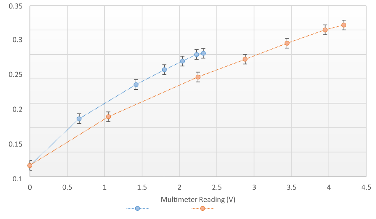
Figure 6: Magnetic Probe Reading and Multimeter Reading for 50 turns and 200 turns Solenoids.
Table 2: Voltage v Magnetic Field for 50 turns solenoid with turn density 555.56 N/m. |
||
| Ammeter (A ± 0.01/A) | Multimeter (V ± 0.01/V) | Magnetic Probe Reading (B ± 0.01/mT) |
| 0.00 | 0.00 | 0.02 |
| 0.19 | 0.66 | 0.12 |
| 0.28 | 1.42 | 0.19 |
| 0.38 | 1.80 | 0.22 |
| 0.39 | 2.04 | 0.24 |
| 0.42 | 2.23 | 0.25 |
| 0.45 | 2.32 | 0.25 |
| Table 3: Voltage v Magnetic Field for 200 turns solenoid with turn density 1052.63 N/m. | ||
| Ammeter (A ± 0.01/A) | Multimeter (V ± 0.01/V) | Magnetic Probe Reading (B ± 0.01/mT) |
| 0.00 | 0.00 | 0.02 |
| 0.14 | 1.05 | 0.12 |
| 0.20 | 2.25 | 0.20 |
| 0.23 | 2.88 | 0.24 |
| 0.26 | 3.44 | 0.27 |
| 0.30 | 3.95 | 0.30 |
| 0.33 | 4.20 | 0.31 |
50-turn solenoid, V = 2.32V, I = 0.37A,
𝐵 = (4𝜋 × 10-7 × 555.56 × 0.37)/ 10-3 (4)
= 0.258 ~ 0.26𝑚𝑇
From 𝑉 = 𝐼𝑅, an increase in voltage across the solenoid with resistance-R would increase current-I, therefore increasing magnetic-field strength. Furthermore, higher turn density corresponds to relatively higher magnetic field strength. Tables 4,5 above indicate that the magnetic probe reading is always lower than the theoretical value of magnetic field strength. The likely reason is that the solenoid converts some of the electric current to heat. This depends on the efficiency of solenoids which has been calculated using the ratio of experimental and theoretical magnetic-field strength.
Table 4: Theoretical and Experimental values of Magnetic Field Strength for 50-turn solenoid. |
|
| Theoretical Magnetic Field Strength (B ± 0.01mT) | Magnetic Probe Reading (B ± 0.01/mT) |
| 0.00 | 0.02 |
| 0.13 | 0.12 |
| 0.20 | 0.19 |
| 0.27 | 0.22 |
| 0.27 | 0.24 |
| 0.29 | 0.25 |
| 0.31 | 0.25 |
| Table 5: Theoretical and Experimental values of the Magnetic Field Strength for 200-turn solenoid. | |
| Theoretical Magnetic Field Strength (B ± 0.01mT) | Magnetic Probe Reading (B ± 0.01/mT) |
| 0.00 | 0.02 |
| 0.19 | 0.12 |
| 0.26 | 0.20 |
| 0.30 | 0.24 |
| 0.34 | 0.27 |
| 0.40 | 0.30 |
| 0.44 | 0.31 |
(5)
(6)
Therefore
(7)
For 50-turn solenoid, V = 2.32V,
(8)
The average % efficiency is calculated for each solenoid below in Tables 6,7.
| Table 6: Average % efficiency of 50-turn solenoid. | ||||
| Theoretical Magnetic Field Strength (B ± 0.01mT) |
Magnetic Probe Reading (B ± 0.01/mT) |
% efficiency | Uncertainty in % efficiency |
Average % efficiency ± 9.52% |
| 0.00 | 0.02 | - | - | 87.42 |
| 0.13 | 0.12 | 92.31 | 16.03 | |
| 0.20 | 0.19 | 95.00 | 10.26 | |
| 0.27 | 0.22 | 81.48 | 8.25 | |
| 0.27 | 0.24 | 88.89 | 7.87 | |
| 0.29 | 0.25 | 86.21 | 7.45 | |
| 0.31 | 0.25 | 80.65 | 7.23 | |
| Table 7: Average % efficiency of 200-turn solenoid. | ||||
| Theoretical Magnetic Field Strength (B ± 0.01mT) |
Magnetic Probe Reading (B ± 0.01/mT) |
% efficiency | Uncertainty in % efficiency |
Average % efficiency ± 7.99% |
| 0.00 | 0.02 | - | - | 74.16 |
| 0.19 | 0.12 | 63.16 | 13.60 | |
| 0.26 | 0.20 | 76.92 | 8.85 | |
| 0.30 | 0.24 | 80.00 | 7.50 | |
| 0.34 | 0.27 | 79.41 | 6.64 | |
| 0.40 | 0.30 | 75.00 | 5.83 | |
| 0.44 | 0.31 | 70.45 | 5.50 | |
For Tables 8,9,
Table 8: Power Generated by 50-turn solenoid. |
||||
| Multimeter (V ± 0.01/V) |
Input Current (Iinput ± 0.01A) |
Output Current (Ioutput) (A) |
Current converted Heat Energy (IH) |
Power (W) |
| 0.00 | 0.00 | 0.00 | 0.00 | 0.00 |
| 0.66 | 0.19 | 0.17 | 0.02 | 0.02 |
| 1.42 | 0.28 | 0.24 | 0.04 | 0.05 |
| 1.80 | 0.38 | 0.33 | 0.05 | 0.09 |
| 2.04 | 0.39 | 0.34 | 0.05 | 0.10 |
| 2.23 | 0.42 | 0.37 | 0.05 | 0.12 |
| 2.32 | 0.45 | 0.39 | 0.06 | 0.13 |
Table 9: Power Generated by 200-turn solenoid. |
||||
| Multimeter (V ± 0.01/V) |
Input Current (Iinput ± 0.01A) |
Output Current (Ioutput) (A) |
Current converted Heat Energy (IH) |
Power (W) |
| 0.00 | 0.00 | 0.00 | 0.00 | 0.00 |
| 1.05 | 0.14 | 0.12 | 0.02 | 0.02 |
| 2.25 | 0.20 | 0.17 | 0.03 | 0.06 |
| 2.88 | 0.23 | 0.20 | 0.03 | 0.08 |
| 3.44 | 0.26 | 0.23 | 0.03 | 0.11 |
| 3.95 | 0.30 | 0.26 | 0.04 | 0.15 |
| 4.20 | 0.33 | 0.29 | 0.04 | 0.17 |
Ioutput (or current used to create magnetic field) = % average efficiency × Iinput (9)
= 87.42 % × 0.45 = 0.39A eq. (10)
Therefore, IH (current converted to heat energy) = Iinput – Ioutput = 0.45 -0.39 = 0.06A
Applying P = VI, where P represents power generated (heat energy per unit time)
P = 0.06 × 2.32 (11)
= 0.14W
c) Heat-Source-Spirit-Lamp: A spirit lamp is used as a heat source. It is lit and placed close to End-A of the test- tube. For each trial, it’s held in place for 2 minutes, measured using a stopwatch (± 0.1s). The drawback of using a spirit lamp is that while it’s strong, the temperature cannot be measured directly. A digital thermometer [least-count (± 0.1 °C)] measured temperature change at End-B.
Fourier’s law of thermal conduction
Fourier’s Law of Thermal Conduction states that the rate of heat transfer through a material is proportional to the (negative) gradient in the temperature and the area. Here the negative sign represents the direction of heat flow [18-29].
The integrated form of Fourier’s Thermal Conduction law:
(11)
Q = Amount of heat supplied
∆𝑡 = Time-duration for which heat is supplied
A = Cross-sectional area (of the tube)
L = Length of tube
∆𝑇𝑒𝑚𝑝 = Temperature-gradient k = Thermal-conductivity constant
Can be written as,
For the experiment, the length (0.15m), cross-sectional area(diameter=0.036m), and the heat supplied by the Spirit-Lamp stay constant.
∆𝑇𝑒𝑚𝑝 = 𝑇END A - 𝑇END B (12)
The heat flows along the temperature gradient, i.e. from hot End-A to relatively cooler End-B. As time passes (2 min), 𝑇END B increases and therefore, ∆𝑇 decreases. From Fourier’s law, it is inferred that decreasing ∆𝑇 results in the thermal conductivity constant ‘k’ increasing. But because nanoparticles are being modelled, the rate of change of 𝑇END B can be interpreted as a measure of the rate of increase of ‘k’.
Enhancement of thermal conductivity
The enhancement factor of thermal conductivity of Nanofluid can be quantified:
𝐸𝑛ℎ𝑎𝑛𝑐𝑒𝑚𝑒𝑛𝑡 𝑓𝑎𝑐𝑡𝑜𝑟 = (𝐾2 / 𝐾1) (13)
K2 = Thermal conductivity constant of nanofluid
K1= Thermal conductivity constant of carrier fluid,
(𝐾2 / 𝐾1) = ‘Thermal conductivity ratio’.
The dependent variable is the temperature which is measured at End-B at regular intervals of 10s. Therefore, the equation is:
(14)
Sample raw data-tables
First, the experiment was conducted under controlled conditions, where no voltage was applied across the solenoid and the test tube contained the ferrofluid and water. Three trials were carried out using each solenoid and Tables 10-13 below show the average initial and final temperatures, the average change, and the rate of temperature change. Those readings are shown when extreme voltages were applied.
Table 10: Temperature Measurements for the 1.05V and 0.12mT readings using a 200-turn solenoid. |
||||||
| Time (s) | Temperature at End B (T ± 0.1 °C) | |||||
| Trial 1 | Trial 2 | Trial 3 | Trial 4 | Trial 5 | Trial 6 | |
| 0.0 | 26.5 | 26.3 | 26.7 | 26.3 | 26.4 | 26.6 |
| 10.0 | 26.5 | 26.3 | 26.7 | 26.4 | 26.4 | 26.7 |
| 20.0 | 26.6 | 26.3 | 26.8 | 26.4 | 26.5 | 26.7 |
| 30.0 | 26.7 | 26.4 | 26.8 | 26.5 | 26.5 | 26.7 |
| 40.0 | 26.9 | 26.6 | 26.9 | 26.6 | 26.6 | 26.8 |
| 50.0 | 27.0 | 26.7 | 27.0 | 26.8 | 26.8 | 26.9 |
| 60.0 | 27.1 | 26.8 | 27.0 | 27.1 | 26.9 | 27.1 |
| 70.0 | 27.3 | 26.9 | 27.2 | 27.3 | 27.0 | 27.3 |
| 80.0 | 27.5 | 27.1 | 27.4 | 27.4 | 27.1 | 27.4 |
| 90.0 | 27.6 | 27.3 | 27.5 | 27.5 | 27.2 | 27.6 |
| 100.0 | 27.8 | 27.5 | 27.7 | 27.7 | 27.4 | 27.8 |
| 110.0 | 28.0 | 27.9 | 27.8 | 27.9 | 27.7 | 27.9 |
| 120.0 | 28.4 | 28.1 | 27.9 | 28.3 | 28.0 | 28.1 |
Table 11: Temperature Measurements for the 4.20V and 0.31mT readings using a 200-turn solenoid. |
||||||
| Time (s) | Temperature at End B (T ± 0.1 °C) | |||||
| Trial 1 | Trial 2 | Trial 3 | Trial 4 | Trial 5 | Trial 6 | |
| 0.0 | 26.4 | 26.7 | 26.8 | 26.5 | 26.6 | 26.3 |
| 10.0 | 26.6 | 26.8 | 26.9 | 26.6 | 26.8 | 26.4 |
| 20.0 | 26.9 | 26.9 | 27.1 | 26.8 | 26.9 | 26.7 |
| 30.0 | 27.3 | 27.3 | 27.4 | 27.0 | 27.2 | 26.8 |
| 40.0 | 27.8 | 27.8 | 27.8 | 27.3 | 27.5 | 27.2 |
| 50.0 | 28.2 | 28.3 | 28.2 | 27.6 | 27.9 | 27.6 |
| 60.0 | 28.7 | 28.9 | 28.5 | 28.1 | 28.5 | 28.3 |
| 70.0 | 29.4 | 29.6 | 29.1 | 28.7 | 29.1 | 28.9 |
| 80.0 | 30.1 | 30.3 | 29.9 | 29.7 | 30.0 | 29.7 |
| 90.0 | 31.2 | 31.0 | 30.8 | 30.8 | 31.0 | 30.7 |
| 100.0 | 32.2 | 32.2 | 31.9 | 31.9 | 32.3 | 31.8 |
| 110.0 | 33.3 | 33.5 | 33.2 | 33.0 | 33.5 | 33.2 |
| 120.0 | 34.7 | 35.2 | 34.9 | 34.2 | 34.7 | 34.6 |
Table 12: Temperature Measurements for the 0.66V and 0.12mT readings using a 50-turn solenoid. |
||||||
| Time (s) ± 0.1 s | Temperature at End B (T ± 0.1 °C) | |||||
| Trial 1 | Trial 2 | Trial 3 | Trial 4 | Trial 5 | Trial 6 | |
| 0.0 | 26.4 | 26.3 | 26.7 | 26.6 | 26.7 | 26.5 |
| 10.0 | 26.6 | 26.4 | 26.8 | 26.7 | 26.8 | 26.7 |
| 20.0 | 26.8 | 26.5 | 27.0 | 26.9 | 27.0 | 26.9 |
| 30.0 | 27.0 | 26.7 | 27.2 | 27.1 | 27.2 | 27.0 |
| 40.0 | 27.3 | 27.0 | 27.5 | 27.4 | 27.4 | 27.2 |
| 50.0 | 27.5 | 27.3 | 27.8 | 27.7 | 27.6 | 27.6 |
| 60.0 | 27.8 | 27.6 | 28.0 | 27.9 | 27.9 | 27.9 |
| 70.0 | 28.1 | 27.8 | 28.2 | 28.3 | 28.2 | 28.2 |
| 80.0 | 28.4 | 28.0 | 28.6 | 28.7 | 28.5 | 28.5 |
| 90.0 | 28.7 | 28.3 | 28.9 | 29.1 | 28.8 | 28.9 |
| 100.0 | 29.0 | 28.6 | 29.2 | 29.4 | 29.2 | 29.2 |
| 110.0 | 29.4 | 28.9 | 29.5 | 29.7 | 29.5 | 29.6 |
| 120.0 | 29.7 | 29.3 | 29.8 | 30.0 | 29.9 | 29.9 |
Table 13: Temperature Measurements for the 2.32V and 0.25mT readings using a 50-turn solenoid. |
||||||
| Time (s) | Temperature at End B (T ± 0.1 °C) | |||||
| Trial 1 | Trial 2 | Trial 3 | Trial 4 | Trial 5 | Trial 6 | |
| 0.0 | 26.1 | 26.5 | 26.4 | 26.3 | 26.6 | 26.3 |
| 10.0 | 26.8 | 27.2 | 27.1 | 27.1 | 27.4 | 26.9 |
| 20.0 | 27.7 | 27.9 | 27.9 | 28.0 | 28.2 | 27.8 |
| 30.0 | 28.9 | 29.0 | 28.7 | 29.1 | 29.6 | 28.8 |
| 40.0 | 30.0 | 30.3 | 30.0 | 30.2 | 30.9 | 29.9 |
| 50.0 | 31.5 | 31.8 | 31.2 | 31.5 | 32.4 | 31.0 |
| 60.0 | 33.2 | 33.5 | 32.6 | 32.9 | 33.8 | 32.4 |
| 70.0 | 35.0 | 35.5 | 34.7 | 34.6 | 35.4 | 34.2 |
| 80.0 | 36.8 | 37.8 | 37.0 | 36.7 | 37.2 | 36.2 |
| 90.0 | 38.9 | 40.3 | 39.9 | 39.1 | 39.4 | 38.5 |
| 100.0 | 41.8 | 42.9 | 42.3 | 42.0 | 42.2 | 41.3 |
| 110.0 | 43.7 | 44.7 | 44.1 | 43.8 | 44.2 | 43.5 |
| 120.0 | 44.7 | 46.0 | 45.3 | 45.3 | 45.7 | 45.1 |
Standard Deviation of Raw Temperature Change Trials at each 10s Interval:
μ represents the mean average temperature at End-B for a given temperature; (15)
N represents the number of voltages, xi represents each data value; σ2 represents the standard deviation (Table 14).
Table 14: Standard Deviation for 6 trials at voltage = 2V for both solenoids. |
||
| Time (s) | Standard Deviation (°C) for 50-Turn solenoid |
Standard Deviation (°C) for 200-Turn solenoid |
| 0 | 0.2 | 0.2 |
| 10 | 0.2 | 0.2 |
| 20 | 0.2 | 0.2 |
| 30 | 0.2 | 0.3 |
| 40 | 0.2 | 0.4 |
| 50 | 0.2 | 0.5 |
| 60 | 0.1 | 0.5 |
| 70 | 0.2 | 0.5 |
| 80 | 0.2 | 0.5 |
| 90 | 0.3 | 0.7 |
| 100 | 0.3 | 0.5 |
| 110 | 0.3 | 0.4 |
| 120 | 0.3 | 0.5 |
Processing of data
The first step in data processing is finding average temperatures recorded after every 10s interval in 6 trials at each voltage and each solenoid (Tables 15,16).
| Table 15: Average Temperature Measurements for each voltage for the 50-turn solenoid. | ||||||
| Time (s) | Average Temperature at End B(T ± 0.1 °C) at each Voltage (V) | |||||
| 0.66V | 1.42V | 1.80V | 2.04V | 2.23V | 2.32V | |
| 0.0 | 26.5 | 26.4 | 26.5 | 26.3 | 26.5 | 26.4 |
| 10.0 | 26.7 | 26.6 | 26.9 | 26.8 | 27.1 | 27.1 |
| 20.0 | 26.9 | 27.4 | 27.3 | 27.3 | 27.8 | 27.9 |
| 30.0 | 27.0 | 27.3 | 27.9 | 28.0 | 28.6 | 29.0 |
| 40.0 | 27.3 | 27.8 | 28.6 | 28.8 | 29.9 | 30.2 |
| 50.0 | 27.6 | 28.2 | 29.3 | 29.7 | 31.1 | 31.6 |
| 60.0 | 27.9 | 28.8 | 30.0 | 30.8 | 32.5 | 33.1 |
| 70.0 | 28.1 | 29.4 | 30.8 | 32.0 | 34.2 | 34.9 |
| 80.0 | 28.5 | 30.0 | 31.7 | 33.3 | 36.0 | 37.0 |
| 90.0 | 28.8 | 30.7 | 32.7 | 34.7 | 38.1 | 39.4 |
| 100.0 | 29.1 | 31.5 | 33.9 | 36.4 | 40.6 | 42.1 |
| 110.0 | 29.4 | 32.3 | 35.1 | 38.2 | 42.4 | 44.0 |
| 120.0 | 29.8 | 33.1 | 36.4 | 40.2 | 43.6 | 45.4 |
| Table 16: Average Temperature Measurements for each voltage for the 200-turn solenoid. | ||||||
| Time (s) | Average Temperature at End B(T ± 0.1 °C) at each Voltage (V) | |||||
| 1.1V | 2.3V | 2.9V | 3.4V | 4.0V | 4.2V | |
| 0.0 | 26.5 | 26.5 | 26.5 | 26.5 | 26.5 | 26.6 |
| 10.0 | 26.5 | 26.6 | 26.6 | 26.5 | 26.6 | 26.7 |
| 20.0 | 26.6 | 26.7 | 26.7 | 26.7 | 26.7 | 26.9 |
| 30.0 | 26.6 | 26.8 | 26.9 | 27.0 | 26.9 | 27.2 |
| 40.0 | 26.7 | 27.1 | 27.2 | 27.3 | 27.2 | 27.6 |
| 50.0 | 26.9 | 27.3 | 27.5 | 27.7 | 27.5 | 28.0 |
| 60.0 | 27.0 | 27.5 | 27.8 | 28.1 | 27.9 | 28.5 |
| 70.0 | 27.2 | 27.8 | 28.1 | 28.5 | 28.3 | 29.1 |
| 80.0 | 27.3 | 28.1 | 28.4 | 28.9 | 28.8 | 30.0 |
| 90.0 | 27.5 | 28.4 | 28.8 | 29.5 | 29.4 | 30.9 |
| 100.0 | 27.7 | 28.7 | 29.2 | 30.0 | 30.1 | 32.1 |
| 110.0 | 27.9 | 29.0 | 29.6 | 30.7 | 31.1 | 33.3 |
| 120.0 | 28.1 | 29.4 | 30.1 | 31.4 | 32.8 | 34.7 |
50-Turn solenoid, voltage=0.66V, B=0.12mT, at the end of 2-minutes:
(16)
𝐴𝑣𝑒𝑟𝑎𝑔𝑒 𝑇𝑒𝑚𝑝𝑒𝑟𝑎𝑡𝑢𝑟𝑒 𝑚𝑒𝑎𝑠𝑢𝑟𝑒𝑑 = 29.8 ± 0.1 °C
Using average initial and final temperatures measured for each voltage, the rate of temperature change will be measured, which is the change in temperature over total time (120s) (Tables 17,18).
| Table 17: Rate of Change of Temperature at End B for different voltages applied across the 200-Turn solenoid. | ||||
| Voltage (V) | Initial Temperature °𝐂 | Final Temperature°𝐂 | Change in Temperature ∆𝐓 ± 𝟎. 𝟐 °𝐂 |
Rate of Change of Temperature °𝐂s-1 |
| 1.05 | 26.5 | 28.1 | 1.6 | 0.013 |
| 2.25 | 26.5 | 29.4 | 2.9 | 0.024 |
| 2.88 | 26.5 | 30.1 | 3.6 | 0.030 |
| 3.44 | 26.5 | 31.4 | 4.9 | 0.041 |
| 3.95 | 26.5 | 32.8 | 6.3 | 0.053 |
| 4.20 | 26.6 | 34.7 | 8.1 | 0.068 |
Table 18: Rate of Change of Temperature at End B for different voltages applied across the 50-Turn solenoid. |
||||
| Voltage (V) | Initial Temperature °𝐂 | Final Temperature°𝐂 | Change in Temperature ∆𝐓 ± 𝟎. 𝟐 °𝐂 |
Rate of Change of Temperature °𝐂s-1 |
| 0.66 | 26.5 | 29.8 | 3.3 | 0.028 |
| 1.42 | 26.4 | 33.1 | 6.7 | 0.056 |
| 1.80 | 26.5 | 36.4 | 9.9 | 0.083 |
| 2.04 | 26.3 | 40.2 | 13.9 | 0.116 |
| 2.23 | 26.5 | 43.6 | 17.1 | 0.143 |
| 2.32 | 26.4 | 45.4 | 19.0 | 0.158 |
∆𝑇𝑒𝑚𝑝𝑒𝑟𝑎𝑡𝑢𝑟𝑒 = 𝐴𝑣𝑒𝑟𝑎𝑔𝑒 𝐹𝑖𝑛𝑎𝑙 𝑇𝑒𝑚𝑝𝑒𝑟𝑎𝑡𝑢𝑟𝑒 − 𝐴𝑣𝑒𝑟𝑎𝑔𝑒 𝐼𝑛𝑖𝑡𝑖𝑎𝑙 𝑇𝑒𝑚𝑝𝑒𝑟𝑎𝑡𝑢𝑟𝑒
(17)
50-Turn solenoid, voltage = 0.66V, B = 0.12mT:
∆𝑇𝑒𝑚𝑝𝑒𝑟𝑎𝑡𝑢𝑟𝑒 = 29.8 − 26.5 = 3.3 °C
Uncertainties get added:
𝑈𝑛𝑐𝑒𝑟𝑡𝑎𝑖𝑛𝑡𝑦 𝑖𝑛 ∆𝑇𝑒𝑚𝑝𝑒𝑟𝑎𝑡𝑢𝑟𝑒 = 0.1 + 0.1 = 0.2 °C
Therefore, ∆𝑇𝑒𝑚𝑝𝑒𝑟𝑎𝑡𝑢𝑟𝑒 = 29.8 − 26.5 = 3.3 °C ± 0.2 °C
(18)
(19)
We can calculate the enhancement factor in the rate of change of temperature, which is theoretically proportional to the enhancement factor in the thermal conductivity of the fluid.
(20)
The experiment was first conducted under controlled conditions, where no voltage was applied and test tubes contained only water and then the Fe2O3-particles with water. Three trials were conducted for each solenoid and Tables 19-21 in the processed data section show the results.
Table 19: Rate of Change of Temperature for both solenoids when no voltage is applied. |
|||||
| Solenoid | Initial Temperature °𝐂 | Final Temperature °𝐂 | Change in Temperature ∆𝐓 ± 𝟎. 𝟐 °𝐂 | Rate of Change of Temperature °𝐂s-1 | Absolute Uncertainty in Rate of Change of Temperature °𝐂s-1 |
| 50 Turn (water) | 26.5 | 28.1 | 1.6 | 0.013 | 0.00168 |
| 50 Turn (Ferrofluid) | 26.5 | 29.4 | 2.9 | 0.024 | 0.00168 |
| 200 Turn (water) | 26.5 | 27.2 | 0.7 | 0.006 | 0.00167 |
| 200 Turn (Ferrofluid) | 26.6 | 27.7 | 1.1 | 0.009 | 0.00164 |
| Table 20: Rates of Change of Temperature and Enhancement factors for the 200-Turn solenoid - with their uncertainties. | |||||
| Rate of Change of Temperature °𝐂s-1 |
Absolute uncertainty in rate °𝐂s-1 |
Percentage uncertainty in rate (%) | Enhancement factor | Absolute Uncertainty in Enhancement factor |
Percentage Uncertainty in enhancement factor (%) |
| 0.013 | 0.00164 | 12.58 | 1.44 | 0.44 | 30.81 |
| 0.024 | 0.00168 | 6.98 | 2.67 | 0.67 | 25.20 |
| 0.03 | 0.00169 | 5.64 | 3.33 | 0.80 | 23.86 |
| 0.041 | 0.00171 | 4.16 | 4.56 | 1.02 | 22.39 |
| 0.053 | 0.00173 | 3.26 | 5.89 | 1.26 | 21.48 |
| 0.068 | 0.00174 | 2.55 | 7.56 | 1.57 | 20.77 |
Table 21: Rates of Change of Temperature and Enhancement factors for the 50-Turn solenoid - with their uncertainties. |
|||||
| Rate of Change of Temperature °𝐂s-1 |
Absolute uncertainty in rate °𝐂s-1 |
Percentage uncertainty in rate (%) | Enhancement factor | Absolute Uncertainty in Enhancement factor |
Percentage Uncertainty in enhancement factor (%) |
| 0.028 | 0.00172 | 6.14 | 1.17 | 0.15 | 13.14 |
| 0.056 | 0.00172 | 3.07 | 2.33 | 0.23 | 10.07 |
| 0.083 | 0.00175 | 2.10 | 3.46 | 0.31 | 9.10 |
| 0.116 | 0.00177 | 1.52 | 4.83 | 0.41 | 8.52 |
| 0.143 | 0.00179 | 1.25 | 5.96 | 0.49 | 8.25 |
| 0.158 | 0.00179 | 1.14 | 6.58 | 0.54 | 8.14 |
Now that we have the ‘𝑅𝑎𝑡𝑒 𝑜𝑓 ∆𝑇𝑒𝑚𝑝𝑒𝑟𝑎𝑡𝑢𝑟𝑒 1’ for each solenoid, we can further calculate the enhancement factor at each voltage.
50-Turn solenoid, voltage = 0.66V, B = 0.12mT:
(21)
Thermal conduction higher in modelled-ferrofluid
Table 12 clearly indicates the thermal-conducting superiority ferrofluids have over water. For both solenoids, the temperature change at End-B was higher when model-Fe2O3-solution was used, even without a magnetic field. In the absence of voltage, the rate of change of temperature for 50 turn-solenoid with water was 0.013 °Cs-1 while it was 0.024 °Cs-1 with Fe2O3-solution. This empirically verifies the fundamental notion of increased heat transfer by a stationary fluid on the dispersion of particles.
Magnetic field’s impact on the temperature measured
Figure 6 demonstrates decreasing trend in B with increasing voltage. For voltage rise 0.66 1.42V, magnetic-probe displayed an increase from 0.12m 0.19mT, with ∆B = 0.07mT. But for voltage rise 2.04 2.23V, B rose from 0.24m 0.25mT only, with ∆B = 0.01mT. While these are significantly less than corresponding theoretical B-values due to the inefficiency of the solenoid, the decrease in magnetic-field strength could be because of the fact that as the voltage applied across the solenoid increased, larger current began flowing through the coils as indicated by Tables 2,3. The larger current would, in time, generate heat energy that would cause the temperature of the coils to increase, thereby increasing the effective resistance of the solenoid. With an increasing variable resistance and constant voltage applied across, the solenoid would tend to decrease the current flowing (𝐼 = v). From B = 𝜇nI, a decrease in I would thus result in decreasing magnetic field strength. This could have been experimentally verified by maintaining a magnetic probe inside the solenoid for the duration of the trials along with a multimeter. The heating of the solenoid was qualitatively observed as the coils were extremely hot to handle after trials taken for larger voltages.
Figure 7 demonstrates that the final temperature of the readings constantly increased with rising B. Rise in temperature can be justified by nanoparticle clustering which supports the magnetic enhancement of thermal conduction. The increase in B would cause the formation of Fe2O3-particle chains which formed conducting bridges, increasing the heat energy transferred from End EndB. Although this has been confirmed in prior studies by Choi and other scientists for iron-oxides of the nano-scale, the model here uses powdered particles ranging in size from 50 𝝁m – 100 𝝁m. Given the greater mass and volume of these particles, the magnetic field strength may not have had the same clustering effect. And there is merit in believing that the temperature rise measured was otherwise caused. The inefficiency of both solenoids generated a weaker-magnetic field with heat energy in coils. In fact, the amount of power- generated as per Tables 8,9 increased with voltage, i.e. B. This heat could have caused a rise in the temperature of the fluid. However, the inner lining of the solenoid was wooden and would have restricted the heat conduction from the coils to the tube. As a result, it cannot be conclusively justified if the temperature rise was due to the magnetic properties of the model ferrofluid or the dissipation of heat.
Figure 7 shows that with every increase in magnetic field strength, ∆T-value constantly increased.
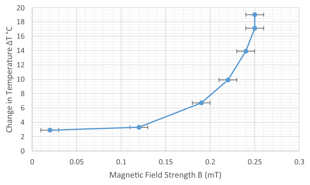
Figure 7: Change in Temperature versus Magnetic Field Strength as measured by the probe for the 50-turn solenoid.
Although it was expected that trend of ∆T would follow that of the magnetic field- strength, the parabolic relation in Figure 7 indicates that although ∆B is decreasing, ∆T increases with a rising slope, indicating the strong effect the magnetic field has on thermal conduction. This could be because the low volume of Fe2O3-particles would tend to align faster even with minor changes in B, thereby increasing the rate of change of temperature as indicated by Table 17,18. However, the last two readings indicate a constant B value (0.25 mT) where the ∆T rises from 17.1 °C 19 °C. This rise in temperature would be due to heat generated by the current in the coils. Further, Figures 8,9 demonstrates a rise in ∆T for every 10s, indicated by an increasing gradient. This means that for every consequent 10s interval, the change in temperature is larger. Since ‘k’ varies inversely with temperature gradient, a decrease in the gradient as temperatures at End-B rise would increase conducting ability of the fluid. Also considering conduction by Fe2O3-particles, aggregation and cluster-formation under a magnetic- field would take time, especially in the model where particles are of the micro-scale in size. Applying the Brownian motion theory, it is perceived that the random motion gradually spreads from End A B. During this time, the kinetic energy of particles closer to End-A would constantly increase, causing a gradual rise in the number of collisions per unit of time. Yet another explanation could be the strength of convection currents developed in water molecules. As the spirit lamp is left lit, the temperature at End-A would also constantly rise, possibly faster than at End-B. Therefore, increasing differences in temperature would gradually strengthen the convectional currents.
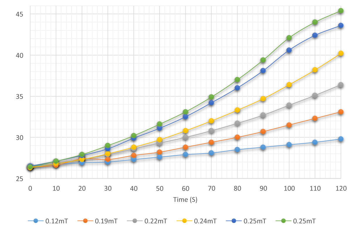
Figure 8: Average Temperature measured at End B versus Time for different magnetic field strengths in the 50-turn solenoid.
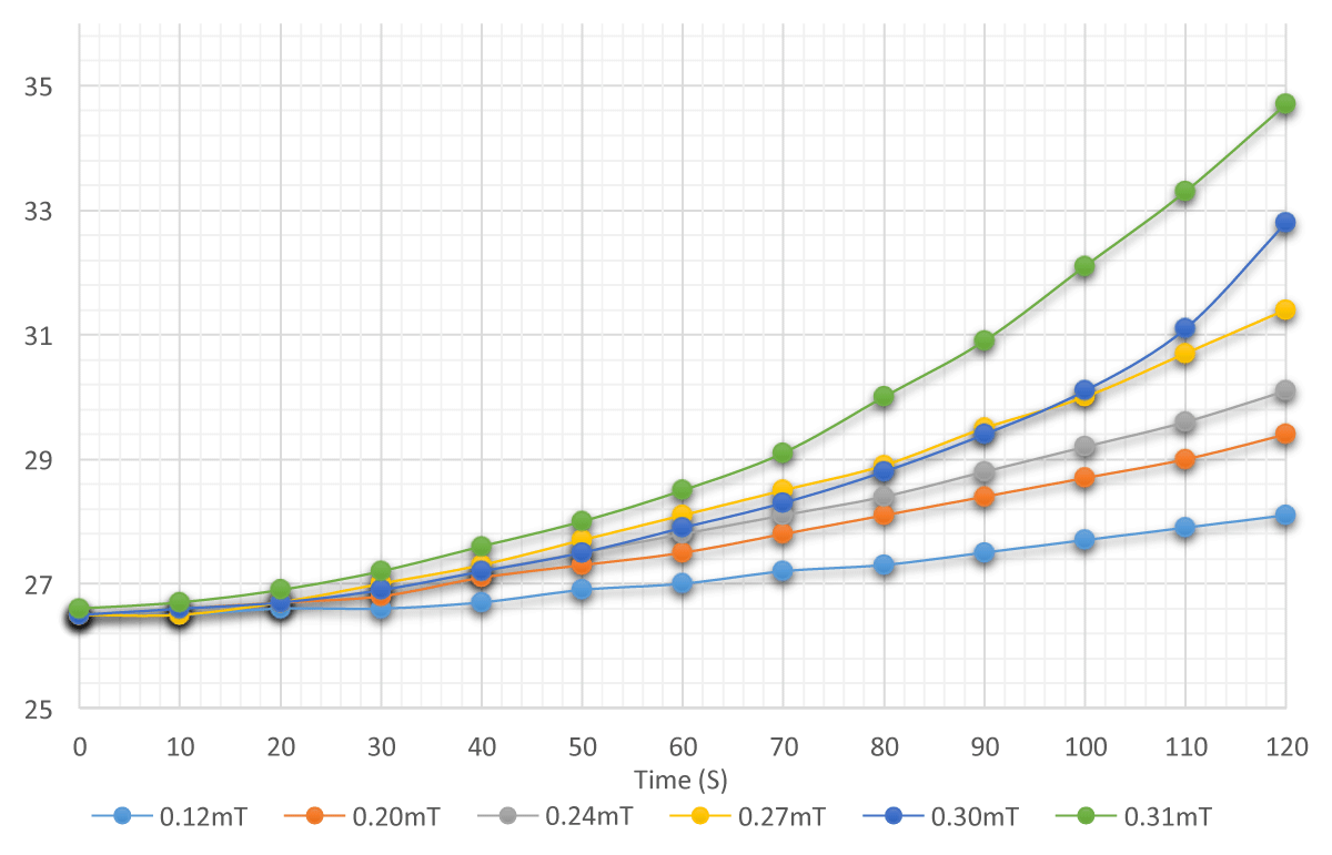
Figure 9: Average Temperature measured at End B versus Time for different magnetic field strengths in the 200 turns solenoid.
For the 50-turn solenoid, the gradient of the curves of 2.23V and 2.32V readings in Figure 8 start decreasing after 100s, when temperatures reach 40 °C. This could be credited to Fe2O3- particles cramping–analogous to the “zippering-effect” due to the clumping of nanoparticles as demonstrated by Figure 2(e)–causing heat conduction in different directions, opposed to the unidirectional heat-flow occurring in linear structures. However, the “clumping” wouldn’t be due to the magnetic field strength but because of the large mass and volume of the Fe2O3- particles.
The results agreed with empirical conclusions drawn up by Wensel J, who used Fe3O4- nanofluids to demonstrate the chain formation using electrostatic forces, working along the Nano-Particle Clustering model. The works of Choi support this chain formation using magnetic fields. The increase in magnetic field observably caused an increase in the rate of temperature- change at the cooler end, with an enhancement factor of the thermal conduction reaching 6 and 7. The variable resistance of solenoids possibly influenced the effective current, thereby affecting the strength of produced magnetic field and heat-dissipated. Therefore, conclusively determined that the enhanced conduction was due to nanoparticle theories and, in part, due to the solenoid’s heat.
- Blums E. Heat and mass transfer phenomena. In: Odenbach S, editor. Ferrofluids: Magnetically Controllable Fluids and Their Applications. Berlin, Heidelberg, New York: Springer-Verlag; 2002.
- Hong TK, Yang HS, Choi CJ. Study of the enhanced thermal conductivity of Fe Nanofluids. Journal of Applied Physics 2005; 97:064311.
- KangH, ZhangT, Yang M, Li L. Molecular Dynamics Simulation on Effect of Nanoparticle Aggregation on Transport Properties of a Nanofluid. J. Nanotechnol. Eng. 2012;3(2):021001. doi:10.1115/1.4007044.
- IUPAC, Compendium of Chemical Terminology, 2nd ed. 1997.
- I Q, Xuan Y, Wang J. Experimental investigations on transport properties of magnetic fluids. Experimental Thermal and Fluid Science 2005; 30:109–16.
- Krichler M, Odenbach S. Thermal conductivity measurements on Ferrofluids with special reference to measuring arrangement. Journal of Magnetism and Magnetic Materials. 2013; 326:85–90.
- Li Q, Xuan Y, Wang J. Experimental investigations on transport properties of magnetic fluids. Experimental Thermal and Fluid Science 2005; 30:109–16.
- Philip J, Shima PD, Raj B. Enhancement of thermal conductivity in magnetite based Nano fluid due to chainlike structures. Applied Physics Letters 2007; 91:203108.
- Sivashanmugam P. Application of Nanofluids in Heat Transfer, An Overview of Heat Transfer Phenomena, Dr. M. Salim Newaz Kazi (Ed.), InTech, DOI: 10.5772/52496. 2012. https://www.intechopen.com/books/an-overview-of-heat-transfer- phenomena/application-of-nanofluids-in-heat-transfer
- Wang X, Mujumdar AS. A review on nanofluids - part I: theoretical and numerical investigations. http://www.scielo.br/scielo.php?script=sci_arttext&pid=S0104-66322008000400001
- Hong TK, Yang HS, Choi CJ. Study of the enhanced thermal conductivity of Fe Nanofluids. Journal of Applied Physic.s 2005; 97:064311.
- Krichler M, Odenbach S. Thermal conductivity measurements on Ferrofluids with special reference to measuring arrangement. Journal of Magnetism and Magnetic Materials. 2013; 326:85–90.
- Li Q, Xuan Y, Wang J. Experimental investigations on transport properties of magnetic fluids. Experimental Thermal and Fluid Science 2005; 30:109–16.
- Godson L. Enhancement of heat transfer using nanofluids—an overview. Renewable and Sustainable Energy Reviews. 2009.
- Brownian Motion: Evidence for Atoms. http://physics.tutorvista.com/thermodynamics/brownian- motion.html
- Philip J, Shima PD, Raj B. Enhancement of thermal conductivity in magnetite based Nano fluid due to chainlike structures. Applied Physics Letters. 2007; 91:203108.
- IUPAC, Compendium of Chemical Terminology. 1997.
- Eapen J, Rusconi R, Piazza R, Yip S. The classical nature of thermal conduction in nanofluids. Journal of Heat Transfer—Transactions of AMSE. 2010;132: 102402.
- Prasher R, Evans W, Meakin P, Fish J, Phelan P, Keblinski P. Effect of aggregation on thermal conduction in colloidal nanofluids. Applied Physics Letters. 2006;89: 143119.
- Nanoscienze e Nanosistemi. http://wwwdisc.chimica.unipd.it/fabrizio.mancin/pubblica/Galileiana/VI%20lezione.pdf
- Kang H, Zhang T, Yang M, Li L. Molecular Dynamics Simulation on Effect of Nanoparticle Aggregation on Transport Properties of a Nanofluid.
- Nanotechnol J. 2012; 3(2):021001. doi:10.1115/1.4007044.
- Guo‐Dong Z, Ji‐Rong W, Long‐Cheng T, Jia‐Yun L, Guo‐Qiao L, Ming‐Qiang Z. Rheological Behaviors of Fumed Silica/Low Molecular Weight Hydroxyl Silicone Oil. Journal of Applied Polymer Science. 2014;131: 40722. 10.1002/app.40722
- Genc S. Heat Transfer of Ferrofluids, Nanofluid Heat and Mass Transfer in Engineering Problems. 2017. DOI: 10.5772/65912. https://www.intechopen.com/books/nanofluid-heat-and- mass-transfer-in-engineering-problems/heat-transfer-of-ferrofluids
- Gutierrez JR. Analysis of thermal conductivity of ferrofluids. Mayaguez: University of Puerto Rico; 2007.
- ME. Mechanical ~ Online Portal for Mechanical Engineers. https://me- mechanicalengineering.com/
- Solenoid. http://hyperphysics.phy-astr.gsu.edu/hbase/magnetic/solenoid.html
- Bhuyan S. Brownian Motion: Definition and examples. Science Facts. 2023. https://www.sciencefacts.net/brownian-motion.html
- Quantitative particle tracking. Leiden University. https://www.universiteitleiden.nl/en/science/physics/biological-matter/daniela-kraft/quantitative-particle-tracking