
More Information
Submitted: December 27, 2023 | Approved: January 18, 2024 | Published: January 19, 2024
How to cite this article: Khan S. Generation of Curved Spacetime in Quantum Field. Int J Phys Res Appl. 2024; 7: 006-009.
DOI: 10.29328/journal.ijpra.1001077
Copyright License: © 2024 Khan S. This is an open access article distributed under the Creative Commons Attribution License, which permits unrestricted use, distribution, and reproduction in any medium, provided the original work is properly cited.
Keywords: Space-time curved, Mikokshi space-time; Stone van Neumann theorem canonical transformation

Generation of Curved Spacetime in Quantum Field
Sarfraj Khan*
Department of Physics, GD. College, Begusarai, LNM University Darbhanga, Bihar, India
*Address for Correspondence: Dr. Sarfraj Khan, Department of Physics, GD. College, Begusarai, LNM University Darbhanga, Bihar, India, Email: [email protected]
To reach such a consistent theory which contains the quantum field theory of particle physics and Einstein’s theory of gravitation as limiting cases, one may proceed in the following way: Standard quantum field theory just ignores the effects of gravity. This is justified in many cases due to the weakness of gravitational interactions at the presently accessible scales. In a first step beyond this approximation, one may consider an external gravitational field that is not influenced by the quantum fields. Here one may think of sources of gravitational fields that are not influenced by the quantum fields under consideration, as high-energy experiments in the gravitational field of the earth or quantum fields in the gravitational field of dark matter and dark energy. This approach amounts to the treatment of quantum field theory on curved spacetimes. The problem of quantization in curved spacetimes is now clearly visible. In Minkowski spacetime, there is a large group of symmetries that enforces a particular choice of vacuum by demanding the vacuum to be invariant. Such a criterion is absent for a general spacetime (M,g). We therefore do not know which state to choose as the vacuum. One might hope that the different prescriptions might be unitarily equivalent such that it doesn’t matter which state one takes to define the theory. Sadly this is not the case: The Stone-Von Neumann theorem is no longer valid for systems with an infinite amount of degrees of freedom. This means that unitarily inequivalent representations of the canonical commutation relations will arise, and it is not clear which equivalence concept representation is the physical one. In the second section of this chapter, we review the notions of Cauchy surfaces and global hyperbolicity.
The general collection of spacetimes is too large for quantum field theory since the notion of causality is important to the setup of the theory. The demand of global hyperbolicity is that spacetime is causally similar to flat space on a global scale. In the third section, we briefly review the generalization of the classical phase space to such a background. The fourth section is devoted to defining the concepts of observers and reference frames. In considering what role observers might play in QFT it is important to have a mathematically rigorous notion of observer. We pose a construction of a local reference frame corresponding to a geodesic observer. The fifth section is allocated to the question of when two different choices of µ give rise to unitarily equivalent QFTs. Sufficient and necessary conditions that are needed to ensure that two theories are equivalent are presented and their proofs sketched. From this, the existence of inequivalent representations can also be seen as these requirements are not satisfied in general. The last two sections of this chapter are allocated to a short review of the Unruh- effect as an example of what can happen in QFT in general spacetimes (although it is set in flat spacetime). First, we review the connection between modes with respect to inertial time and ones with respect to accelerated time. This leads to the result that the Minkowski vacuum is a thermal state with respect to the Rindler-quantization. After this, we investigate the reality of this thermal bath by coupling the system to a model particle detector, which sheds some light on the interpretation of QFT as a theory of particles.
Global hyperbolicity and space-time splits
Since we already did a lot of the work involved in the quantization of the free scalar field the rest of the task is now fairly straightforward. As a first task, we need to generalize the classical space of solutions to more general spaces. In order to do this we need to single out some spacetimes that are sufficiently nice for the wave-equation to have solutions.
Let (M, g) be some four-dimensional spacetime with metric signature (−, +, +, +). Throughout this thesis, we will assume spacetime to be time-oriented: a global choice for ’future-pointing’ has been made. The metric tensor g is abstractly defined as a map sending two vector fields to a smooth, real function in spacetime. In terms of components this is given by the contraction of indices:
g(X, Y)(x) = gµν(x)Xµ
(x)Yν(x), where X and Y are vector fields and x ∈ M.
For each spacelike subset S ∈ M we can define the timelike future of the set as
I+(S) = {x ∈ M | There is a future pointing timelike curve connecting S to x}.
We likewise define the timelike past of S. By causal we will always mean: timelike or lightlike. Hence we also define the causal past/future J ±(S) of S as the sets of all points causally connected to S in the past/future. These sets are usually interpreted as all events that can be influenced by events in S since light signals travel along lightlike paths. Related to this is the definition of the domain of dependence of the set S. This is the set of events that is completely and uniquely influenced by S. We define it as:
D+(S) = {x ∈ M | every past-pointing causal curve without past endpoint through x intersects S}, with D−(S) defined similarly and
D(S) = D+(S)∪D−(S).
We see that any information reaching a point in D+(S) must also register on S, and any information leaving a point in D−(S) also does. Concretely: If we know what happens on S, we can infer all that happens in D(S). We exclude curves with a past endpoint since we want to prevent points from falling outside of D(S) simply because we stopped the curves through x before hitting S. The extra demand that we will put on our spacetimes is that some closed surface Σ exists that is large enough to capture all that happens in M. Concretely, we call a smooth, closed, achronal set Σ ∈ M a Cauchy surface if D(Σ) = M. It follows that every inextendible causal curve in M hits Σ exactly once. We call a spacetime Figure 1: The left figure shows the timelike past/future of the closed set S. The causal past/future J±(S) is the union of the enclosed volume with the dashed boundaries. The right figure shows the past/future domain of dependence of S. Note that these sets are always contained within the causal past/future, but are in general a lot smaller.
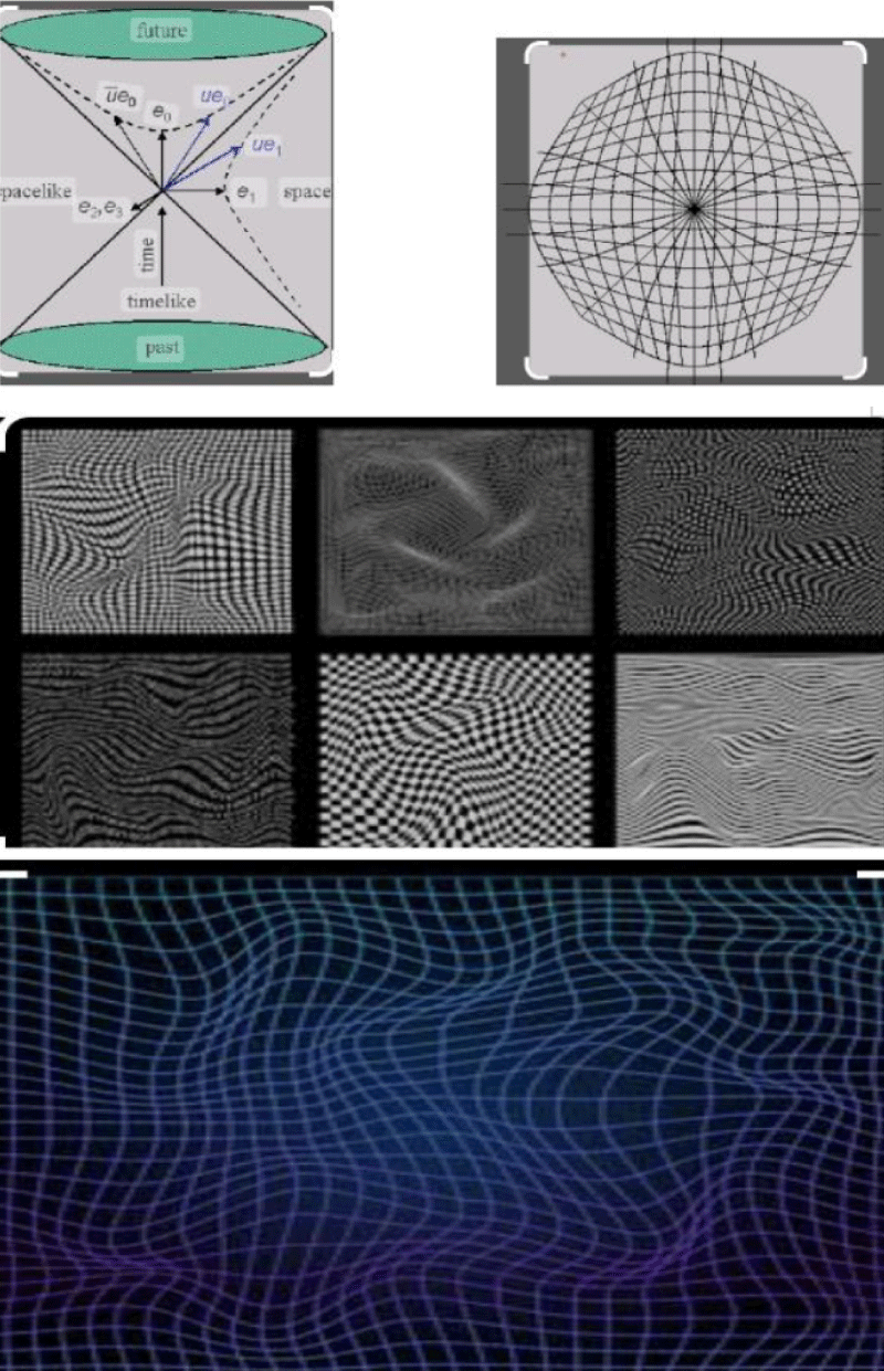
Figure 1:
A classic theorem by Geroch [1] states that on a globally hyperbolic spacetime, we can always find a global time function, ie. A smooth function increasing on any future-directed curve whose gradient is nowhere zero. Every surface of constant time will then be a Cauchy surface. As such the topology of globally hyperbolic spacetimes is particularly simple, it is homeomorphic to R × Σ for some 3-manifold Σ. Proof of this fact can be found in the proposition [2-10].
This implies that a globally hyperbolic spacetime admits a foliation. A foliation is a global decomposition of spacetime into space and time. Concretely, it is a collection of smooth hypersurfaces Σt (which all have the same topology) labeled by a time-coordinate t such that the Σt’s together cover the entire manifold, whilst no two different surfaces intersect. We can define a time function at a point by looking at which unique Σt the point is part of. We can find coordinates adapted to the foliation as follows. If we choose spatial coordinates {xi} on (a patch of) Σt for i = 1, 2, 3 then {t, xi} forms a coordinate chart for M. This gives a basis for the tangent space: {∂t, ∂i}. The vector field ∂t connects the different slices of the foliation but is in general not normal to the hypersurface Σt. This is because transport along this vector does not necessarily leave the spatial coordinates invariant. Hence we can decompose it into parts that are normal and tangential to
Σt∂t = αN + β
Here N is the future-directed unit normal to Σt. We call α the lapse of the coordinate system, which is a scalar. The tangential part β is called the shift and is a spacelike vector. Loosely speaking the lapse indicates how far away a neighboring hypersurface of constant time is, and the shift indicates how far one has to move the coordinates around in going to this surface. A straightforward calculation of the metric components in this coordinate chart gives:
gµν = −α 2 + (β+iβ)/ i βj
βi /hij
Where hij is the spatial metric induced on the tangent space of Σt by g in the coordinates {xi}. The inverse metric can then be calculated:
µν =(−1α2β+j/α2 -βiα2 h+ ij −iβjα2!)
The purpose of this formalism is to split spacetime into space and time separately. The covariant picture of space and time being the same is mathematically elegant but often not very practical in calculations. Choosing a Cauchy surface, a lapse and a shift effectively unravels the union of space and time. If coordinates are chosen such that β vanishes, the spacetime metric takes a form where space and time are not mixed at all. It should be clear that these choices are not unique: We can slice spacetime in many different ways, and when we have done so there are many different choices for lapse and shift that are available. As such, no dependence of physical observables on these choices is allowed.
Generalization of the classical phase space
We now continue to the covariant generalization of the classical field system. Clearly, we should swap out the partial derivatives for covariant derivatives in order to obtain a covariant equation. In fact, it is only because we posed the Klein-Gordon equation in Cartesian coordinates that we did not need to do so before because in the flat case, the of Christoffel symbols vanish and covariant and partial derivatives are the same. From this point onward, we will always use the symbol ∇ to denote covariant derivatives, and the KG-equation becomes 1
:(gµν∇µ∇ν − m2)φ = (2 − m2)φ = 0, (3.5)
Where the d’Alembertian operator is defined by 2 = gµν∇µ∇ν. We have the following theorem, originally due to Leray:
Theorem: Let (M, g) be a globally hyperbolic spacetime with Cauchy surface Σ and let N be the normal vector to Σ. If φ and π are two smooth functions on Σ supported within some compact subset K then there is a unique smooth solution ψ to the KG-equation such that ψ|Σ = φ and Nµ∇µψ|Σ = π. This solution has compact support on any other Cauchy surface and is supported in
J+(K) ∩ J −(K). Furthermore, if
We vary the initial conditions outside of some closed subset S of Σ then the solution remains unchanged within D(S).
For proof of this theorem, we refer to [2] (Wald, 1984). A self-contained treatment of wave equations in curved spacetimes can be found in (Bar, Ginoux, and Pfaffle, 2007). The theorem above states that in a globally hyperbolic spacetime solutions to the KG equation are uniquely characterized by their footprint on a Cauchy surface, and that this information is enough to reconstruct the solution. The propagation of information is causal the potential term admits a new term of the right physical dimensions, namely some constant times the Ricci scalar. This is often added with prefactor since this renders the equation conformally invariant. This allows many interesting examples to be explicitly calculated in conformally flat spacetimes. We will not add it here, for the reason that it adds little to the discussion and we see no reason to introduce some extra coupling to gravity on top of changing the background metric to a curved one in the sense that was discussed above. In the previous chapter, we described solutions to the KG-equation by the initial data they have at t = 0. Clearly, the set t = 0 is a 3-surface in Minkowski space that hits every causal curve exactly once, and hence it is a Cauchy surface. The theorem above generalizes this: In a globally hyperbolic spacetime we pick some Cauchy surface Σ and set
V = C∞c(Σ)MC∞c(Σ)
Consisting of pairs (φ, π) of smooth functions of compact support on Σ. From the above theorem it follows that it is not important which Σ we take: If we take some compactly supported smooth initial conditions on one Cauchy surface, it uniquely hinders smooth compactly supported data on any other. The symplectic form is gen-eralized to
σ((φ1, π1),(φ2, π2)) = ZΣ(π1φ2 − π2φ1)√hd3x
By the theorem above, there is a one-to-one correspondence between V and solutions to the wave equation. If we make this identification between ψ and (φ, π) the symplectic form reads
σ(ψ1, ψ2) = Z
Σ(ψ1←→∇µψ2)dΣµ
Here dΣµ = Nµ√hd3x
Is the surface measure of Σ, where Nµ is the future pointing normal vector to Σ and h is the determinant of the spatial metric. We can use Gauss’s theorem to see that this does not depend on the Cauchy surface that is used: Suppose we have Σ1, Σ2 Cauchy surfaces and denote the volume enclosed by Ω, then Gauss’s theorem gives us the equality:
σ1(ψ1, ψ2) − σ2(ψ1, ψ2) = ZΩ∇µ(ψ1←→∇µψ2) = ZΩψ1(m2 − m2)ψ2 = 0 (3.9)
This gives us two equivalent ways of looking at the classical phase space. These constructions use 3-dimensional test functions to smear the quantum field such that it is well-defined. An equivalent construction is to use 4-dimensional test functions, and will sometimes also take this viewpoint. Thus, look at the space of 4-dimensional test functions C∞0
(M) of smooth functions of compact support on spacetime. This construction makes use of the fact that for
f ∈ C∞0
(M) we can solve the Klein-Gordon equation with source f. The retarded and advanced solutions are defined by
(2 − m2)Rf = f,(2 − m2)Af = f, (3.10)
Where Rf = 0 outside of the future of the support of f, and Af = 0 outside of the past of the support. Then (A − R)f = Ef is a solution to the homogeneous wave equation, which registers compactly on any Cauchy surface because the support of f is compact. Hence we find that E is a map of C∞ 0 (M) → V. One can show (Wald 1995) that this map is surjective, and that its kernel is exactly the image of (2−m2 ). Hence we find
V ∼= C∞c(M)/(2 − m2)C∞c(M).
The interpretation of a reference frame is that it represents a collection of fictitious observers that can work together in order to establish non-local measurements. A reference frame is called synchronizable if functions t and h on M exist such that X = −h∇t, and we call it proper time synchronizable if we can choose h = 1. These reference frames allow the different observers in the frame to synchronize their clocks 4 and define surfaces of constant time t. This affects a spacetime split: The observers agree that the surfaces of constant t form space and global time is equal to each observer's proper time. This is the best-case scenario, but we are not guaranteed the existence of a unique global synchronizable reference frame containing γ. Clearly, the concept of a reference frame is a global notion: Vector fields are defined on the whole of spacetime and are sensitive to the global properties of the manifold. As such it would be too optimistic to expect an observer to induce a unique reference frame that he is one of the observers of. In general, there will be many different reference frames that extrapolate a single observer γ. To restrict this choice, we can ask for some criterion to be satisfied which implements the idea that the reference frame ’behaves like the observer γ’. For example, since will be looking at geodesic observers it would be natural to ask for a reference frame which is geodesic 5. However, because gravity is attractive, geodesics are likely to cross and such a reference frame will not exist in any realistic model. The problem is that, while there are many extensions of a single observer to a reference frame, there are in general no global extensions with nice properties. We can, however, locally define reference frames around the worldline of the observer. While this does not yield the full notion of a reference frame, we would argue that this notion is unphysical. A realistic observer cannot measure anything that has a large spatial separation from his own worldline. Cooperation between multiple observers can increase the range of measurements that can be performed, but this would always require different observers to communicate to compare their findings. This can only be done meaningfully if the different observers can synchronize their clocks since then they can compare their measurements with an agreement to when they were made. There are schemes for synchronizing clocks between observers, such as the radar method. These methods are, however, not globally applicable we therefore take the viewpoint that a realistic reference frame should always be lo-cally defined on some open set inside M which contains part of γ. This corresponds to the idea that the observer is able to operate some spatially extended apparatus to perform measurements away from the exact position of his worldline and that he could communicate with other observers who are close. Finally in this paper theoretical study of different types and generations of spacetime curved in Mikokshi and other Hilbert space and multiple dimensional vectors spacetime curved.
- Geroch R. Domain of dependence. Journal of Mathematical Physics. 1970; 11: 437–449.
- Hawking SW, Ellis GFR. The Large Scale Structure of Space–Time. Cambridge: Cambridge University Press. 1973; 1. doi: 10.1017/CBO9780511524646.
- Fulling SA. Remarks on positive frequency and Hamiltonians in expanding universes. General Relativity and Gravitation. 1979; 807–824. doi: 10.1007/BF00756661.
- Fulling SA, Narcowich FJ, Wald RM. Singularity structure of the two-point function in quantum field theory in curved spacetime II. Annals of Physics. 136: 243-272.
- Fulling SA. Nonuniqueness of canonical field quantization in rieman- nian space-time. Physical Review D. 1973; 7:2850–2862. doi:10.1103/PhysRevD.7.2850.
- Fulling SA, Sweeny M, Wald RM. Singularity struc- ture of the two-point function in quantum field theory in curved spacetime. Communications in Mathematical Physics. 1978; 63: 257-264. doi: 1007/BF01196934. URL: http://link.springer.com/10.1007/BF01196934.
- Stefan H, Wald RM. Quantum fields in curved spacetime. General Relativity and Gravitation: A Centennial Perspective. 2015; 513–552. doi: 10.1017/CBO9781139583961.015. arXiv: 1401.2026.
- Wolfgang J, Schrohe E. Adiabatic vacuum states on general space-time manifolds: Definition, construction, and physical properties. An- nales Henri Poincare. 2002; 3:1113-1182. doi: 10.1007/s000230200001. arXiv: math-ph/0109010 [math-ph].
- Kay BS. Linear spin-zero quantum fields in external gravitational and scalar fields. Communications in Mathematical Physics. 1980; 71: 29-46. doi:10.1007/BF01230084. http://link.springer.com/10. 1007/BF01230084.
- Kay BS. The double-wedge algebra for quantum fields on Schwarzschild and Minkowski spacetimes. Communications in Mathematical Physics. 1985; 100: 57–81.