
More Information
Submitted: May 12, 2026 | Accepted: May 29, 2026 | Published: June 01, 2026
Citation: Cojocaru AV, Balint S. Mirroring the Rosehip-neuron Cell Behavior in the Continuous-time Artificial Hopfield Neural Network. What Problems Arise? Int J Phys Res Appl. 2026; 9(6): 162-189. Available from:
https://dx.doi.org/10.29328/journal.ijpra.1001155
DOI: 10.29328/journal.ijpra.1001155
Copyright license: © 2026 Cojocaru AV, et al. This is an open access article distributed under the Creative Commons Attribution License, which permits unrestricted use, distribution, and reproduction in any medium, provided the original work is properly cited.

Mirroring the Rosehip-neuron Cell Behavior in the Continuous-time Artificial Hopfield Neural Network. What Problems Arise?
Andreea V Cojocaru* and Stefan Balint
Department of Computer Science, West University of Timisoara, Blvd. V. Parvan 4, 300223 Timisoara, Romania
*Address for Correspondence: Andreea V Cojocaru, Department of Computer Science, West University of Timisoara, Blvd. V. Parvan 4, 300223 Timisoara, Romania, Email: candreeavalentina@gmail.com
This paper, provide a mirroring of the voltage dynamics of a rosehip nervous cell in the framework of the continuous-time Hopfield artificial neural network. The aim is to identify, those elements which can explain the empirically established properties of the biologic rosehip-neuron.
In the real world, there are biological neural systems and artificial neural systems. For the biological ones, the mathematical framework was developed by Hodgkin-Huxley (Nobel Prize in 1963), and for the artificial ones, it was developed by Hopfield (Nobel Prize in 2024). The aim of our paper is to analyze how the behavior of a neural network composed of rosehip biological cells is reflected in a Hopfield-type artificial neural network model. This aim is not just an academic curiosity, considering the fact that measurements in the case of rosehip biological cells are also made using artificial neural networks.
Rosehip neurons are inhibitory GABAergic neurons, present in the first layer (the molecular layer) of the human cerebral cortex. They make up about 10-15% of all inhibitory neurons in Layer 1 [1]. Neurons of this type (having "large ‘rosehip’-like axonal boutons and compact arborization") exist in humans, but have not been reported in rodents [2]. Rosehip neurons are named after the rose hip fruit due to the axon terminal's resemblance to their berries. These rosehip cells show an immunohistochemical profile (GAD1+CCK+, CNR1–SST–CALB2– PVALB–) matching a single transcriptomically defined cell type whose specific molecular marker signature is not seen in mouse cortex. Rosehip cells in layer 1 make homotypic gap junctions, predominantly target apical dendritic shafts of layer 3 pyramidal neurons, and inhibit back propagating pyramidal action potentials in micro domains of the dendritic tuft (Figure 1.1).
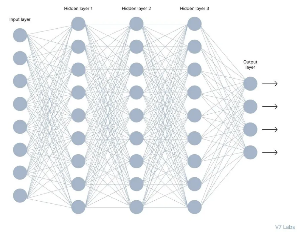
Figure 1.1: Neural network.
These cells are therefore positioned for potent local control of distal dendritic computation in cortical pyramidal neurons (Figure 1.2).
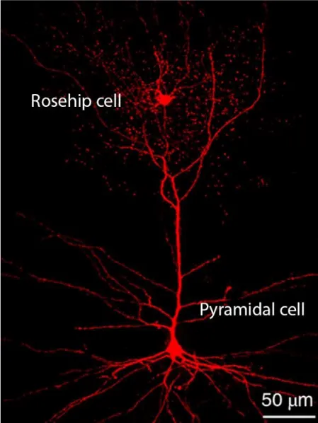
Figure 1.2: Rosehip and pyramidal nervous cell.
An international group of scientists discovered Rosehip neurons and announced their discovery in August 2018. These authors contributed equally to this work: Eszter Boldog (University of Szeged, Szeged, Hungary), Trygve E. Bakken (Allen Institute for Brain Science, Seattle, WA, United States), and Rebecca D. Hodge (Allen Institute for Brain Science, Seattle, WA, United States). They identified this cell with the help of RNA sequencing [2] (Figure 1.3).

Figure 1.3: John Joseph Hopfield delivering his lecture at the 2024 Nobel Prize lectures.
Continuous-time artificial Hopfield neural networks claims to be mathematical descriptions of voltage propagation appearing in artificial neural networks. If this description is appropriate also for the description of voltage propagation in biological nervous system, then the voltage propagation in a rosehip nervous cell has to be mirrored with accuracy in the artificial Hopfield neural network. For instance, it has to mirror that rosehip nervous cell inhibit back propagating pyramidal action potentials in micro domains of the dendritic tuft. The aim of this paper is, to identify those elements concerning the voltage propagation in a continuous-time artificial Hopfield neural network, which can explain the empirically established properties of the biologic rosehip-neuron or underline the problem which arise.
A continuous-time artificial Hopfield neural network, describing the voltage evolution in an artificial neural network of n neurons, is a system of nonlinear differential equations of the form
(1.1)
where: ai > 0, Ii are constants, ai is related to the neuron i membrane capacity and Ii is related to the external electrical input, is a constant matrix referred to as the interconnection matrix, gj: R→ R, j = 1…n represent the neuron j input-output activation function. (see [3] pg.173 formula (5.1)) An activation function gj is a mathematical “gate” between the input feeding the neuron j and its output going to the next neuron. Decides whether neuron j should be activated or not. This means that it will decide whether the neuron’s j input to the network is important or not in the process of prediction using simpler mathematical operations. The input-output activation functions are used to calculate some intermediate function in the hidden layer, which is then used to calculate an output. In literature frequently the next 12 input-output activation functions appear (Figure 1.4).
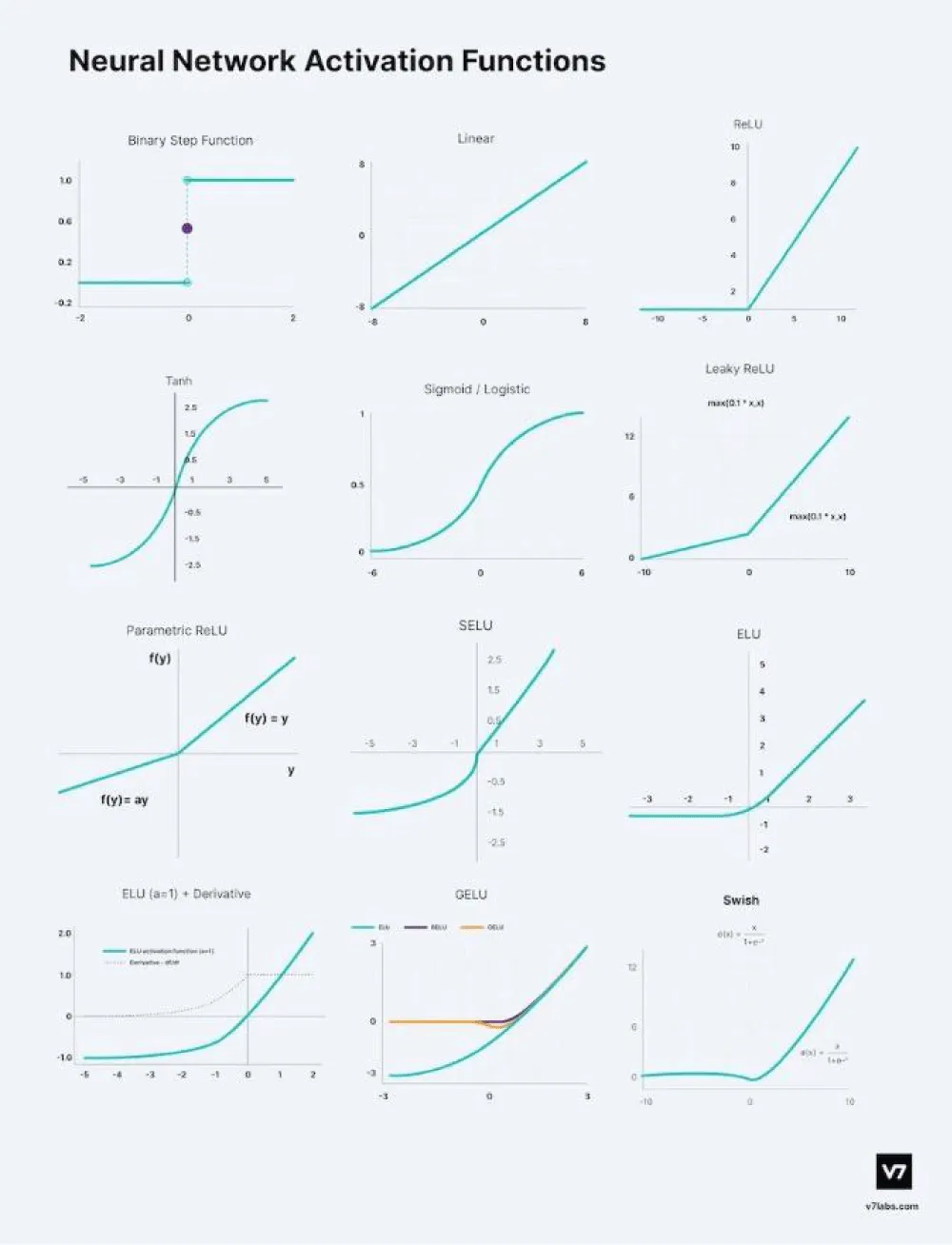
Figure 1.4: Input-output activation functions used in computations.
The system (1.1) can be written in matrix form:
(1.2)
Where , , and is given by .
Let be the function given by . With this function equation (1.2) can be written in the form:
(1.3)
By definition a rest state of (1.3) is a solution of the equation:
(1.4)
In other words a rest state of the system is an element X0 from Rn which verifies (1.4). A rest state X0 (if exist) then X0 is called ‘rest potential’ The name ‘rest potential X0’ is justified by the fact that if I is equal to 0 then the solution of (1.3) which verifies the initial condition is constant equal to X0. According to [3] given voltage state X is rest state if and only if it is solution of the nonlinear algebraic equation:
(1.5)
Theoretically it can happen that the equation (1.5) has no solution, has one solution, or there exits several different voltage states Xj, j = 1… m which are solutions for (1.5).
2. Existence, uniqueness and dependence of the transfer coefficient T on the membrane capacity, and on the input output activation function in case of a single rosehip nervous cell, according to the artificial Hopfield neural network
For a single rosehip nervous cell, the system of differential equations (1.1) becomes
(2.1)
A given voltage state x0 is a rest state if it is solution of the next equation
(2.2)
Therefore, for a given input-output function g(x) according to (2.2), if g(x0) ≠ 0 then, the transfer coefficient T is given by:
(2.3)
If g(x0) = 0, then according to (2.2), x0 = 0. Therefore, in case of a rest state x0 ≠ 0 an input–output function g for which g(x0) = 0, is not appropriate for use. The physical reason is that there is no feedback. For this reason, in case of a rest state x0 ≠ 0 we will consider only input–output function g for which g(x0) ≠ 0.
i). Concerning the numerical value of the rosehip nervous cell membrane capacity Cm, in scientific literature is estimated to be in the range [50,150] [pF]=[50 × 10-12, 150 × 10-12][F] and is estimated to be in the range [1.36 × 10², 2.70 × 10²][s]-1.
ii). For the rosehip nervous cell, the rest potential x0, in scientific literature, is estimated to be around -70 [mV] = -70 ×10-3 [V]
Therefore, for a given input-output function g(x), for which g(-70×10-3) ≠ 0, according to (2.3), the transfer coefficient T is given by:
(2.4)
It follows that:
- in case of rosehip nervous cell the so called ‘ReLU’ input- output function g(x) = max (0,x) is not appropriate for use, because g(-70 × 10-3) = max (0, -70×10-3) = 0 (no feedback).-in case of rosehip nervous cell the so called ‘Dying ReLU’ function g(x) = 0 for, x < 0 and g(x) = 1 for, x ≥ 0 is not an appropriate input-output function to be used, because g(-70 × 10-3) = 0 (no feedback).
-in case of the rosehip cell the so called ‘Binary Step Function’ defined as: g(x) = 0 for x ≤ 0 and g(x) = 1 for x > 0, is not an appropriate input-output function to be used because g(-70 × 10-3) = 0 (no feedback).
-for the so called ‘Sigmoid/Logistic’ input-output function ; T ∈ [-39.17040462, -19.73027788] and T varies according to the next Figure 2.1.
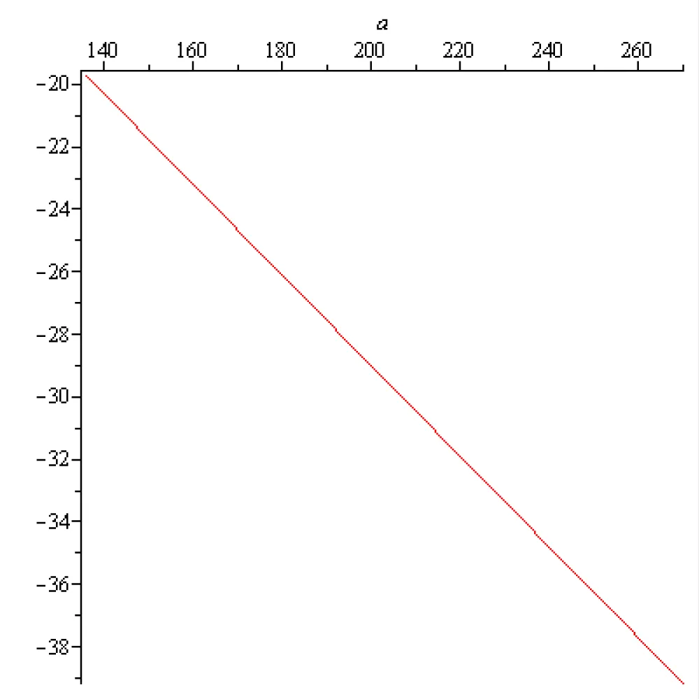
Figure 2.1: T versus a for .
The sign minus physical meaning in this context is negative feedback (self-inhibition). It is related to instability. If T is negative, the rest state is unstable i.e., the rosehip cell voltage, is no longer an energy minimum. The cell state tends to "run away" from the current state. For the initial state x0 = -70 × 10-3[V] and for two membrane ‘capacities’ a = 136[s]-1 and a = 270[s]-1 this "run away" dynamics is represented with red and green colors respectively, on the next Figure 2.2, 2.3 and 2.4:
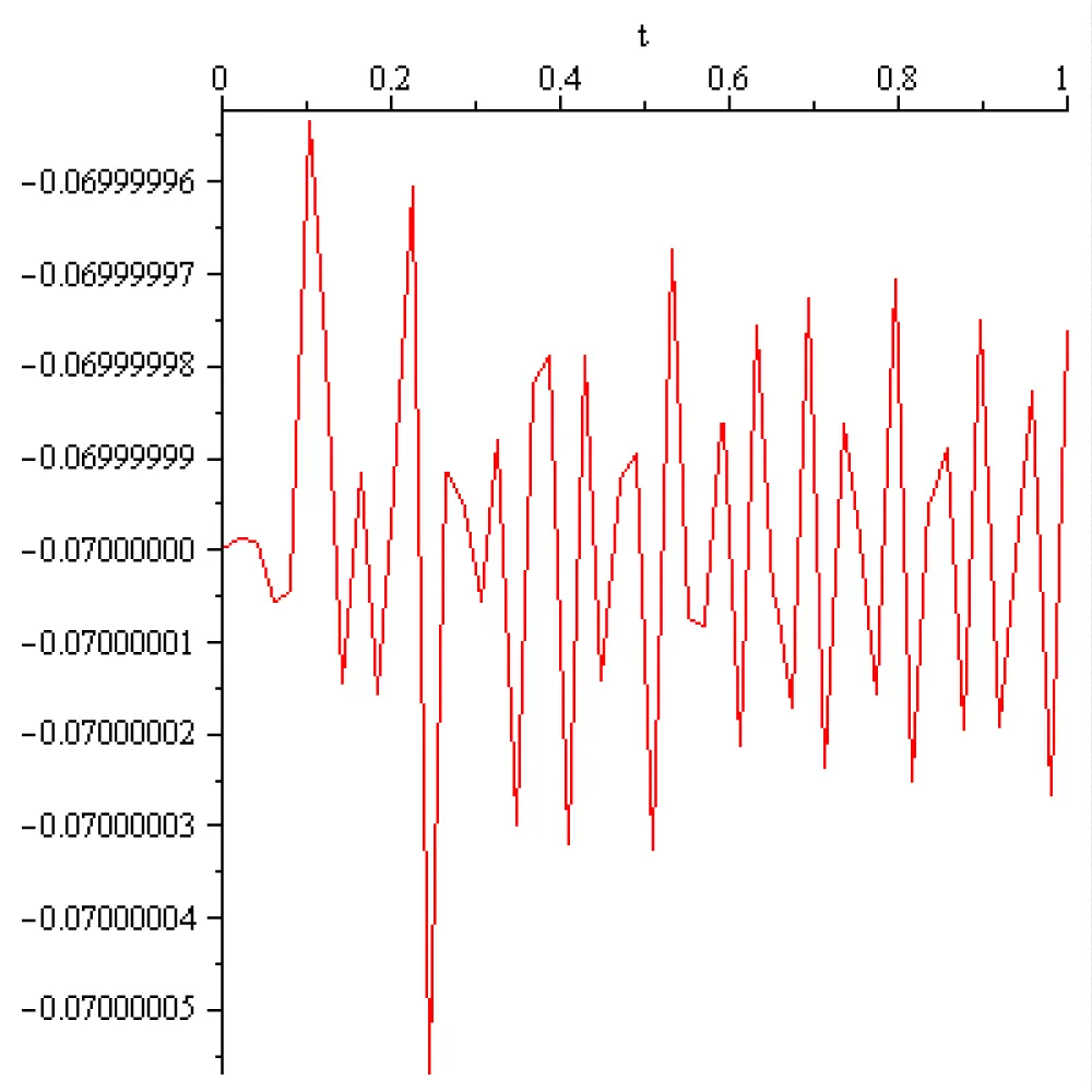
Figure 2.2: T = −19.73027788.
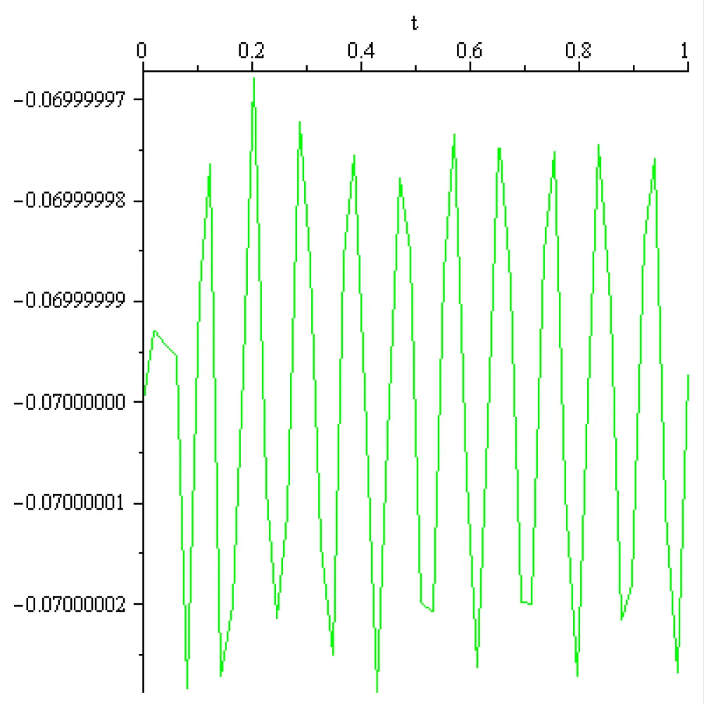
Figure 2.3: T = -39.17040462.
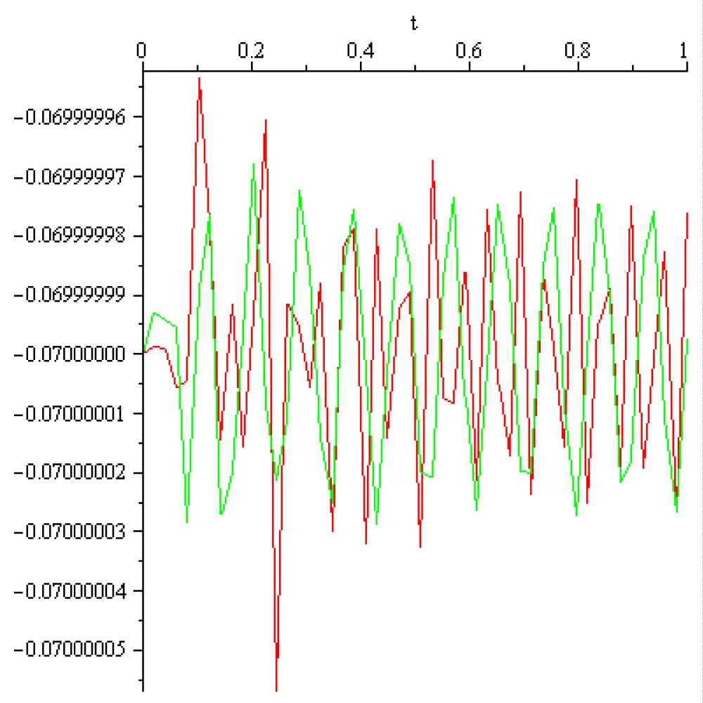
Figure 2.4: T = −19.73027788.
- for the ‘Sigmoid*(1-Sigmoid)’ input-output function , T ∈ [-75.69264780, -38.12666704] and T varies according to the next Figure 2.5.
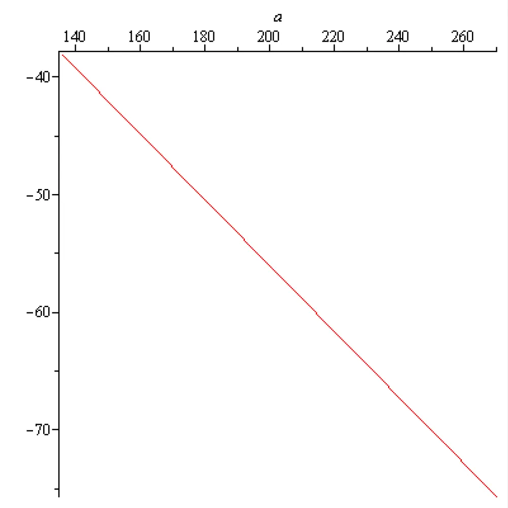
Figure 2.5: T versus a, for .
The sign minus physical meaning in this context is negative feedback (self-inhibition). It is related to instability. If T is negative, the rest state is unstable i.e., the rosehip cell voltage is no longer an energy minimum. The cell state tends to "run away" from the current state. For the initial state x0 = -70 × 10-3[V] and for two membrane ‘capacities’ a = 136[s]-1 and a = 270[s]-1 this "run away" dynamics is represented, with red and green colors respectively on the next Figure 2.6, 2.7 and 2.8:
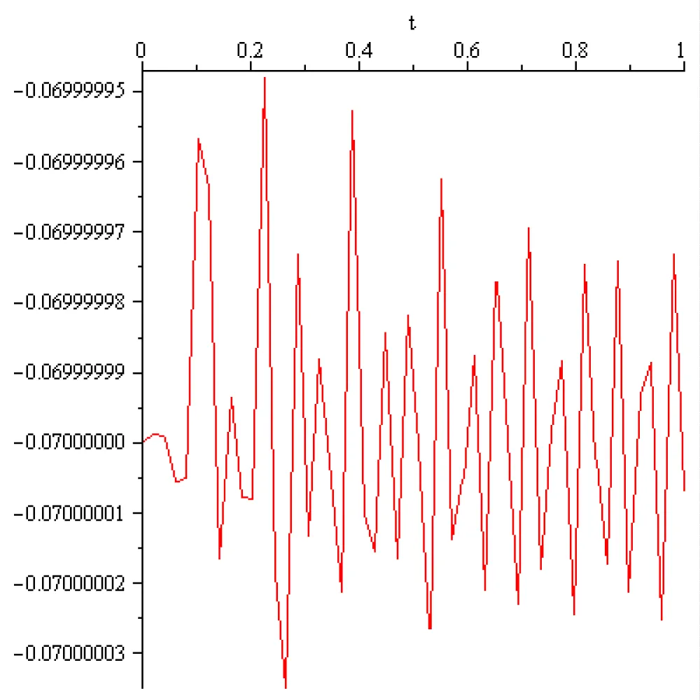
Figure 2.6: T = −38.12666704.
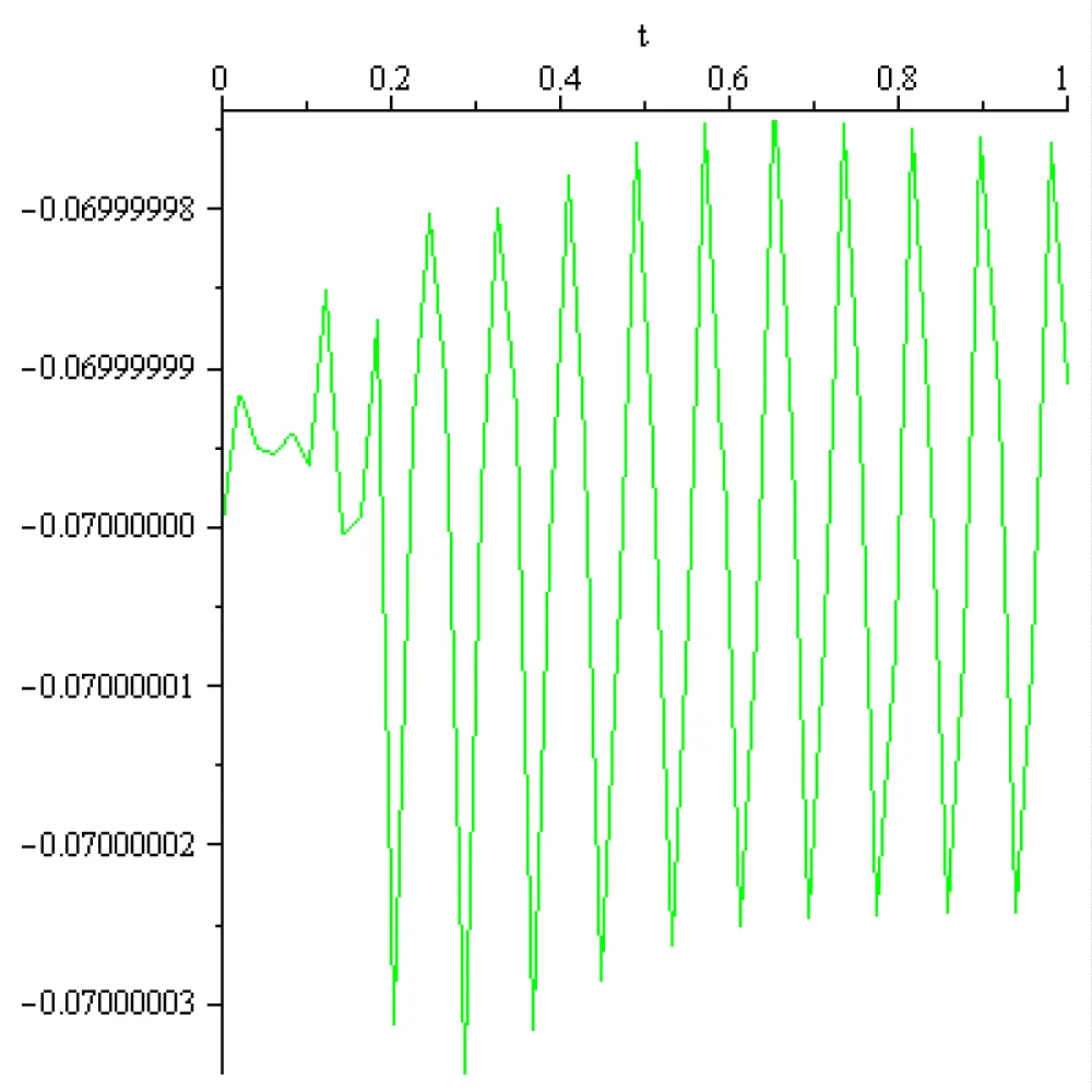
Figure 2.7: T = −75.69264780.
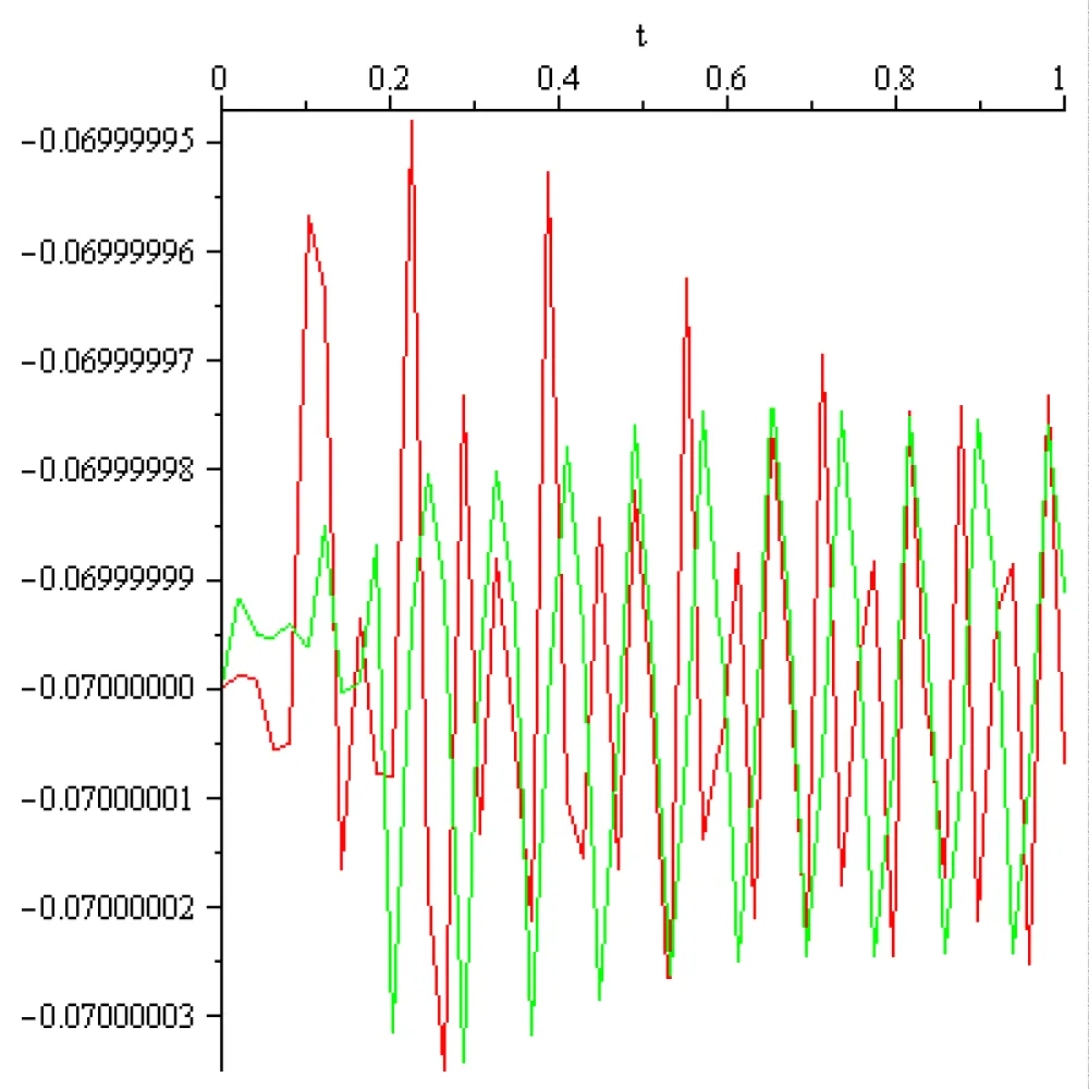
Figure 2.8: T = −38.12666704.
-for the ‘Tanh derivative’ input-output function , T ∈ [-9.566724239, -18.99276136] and T varies according to the next Figure 2.9.
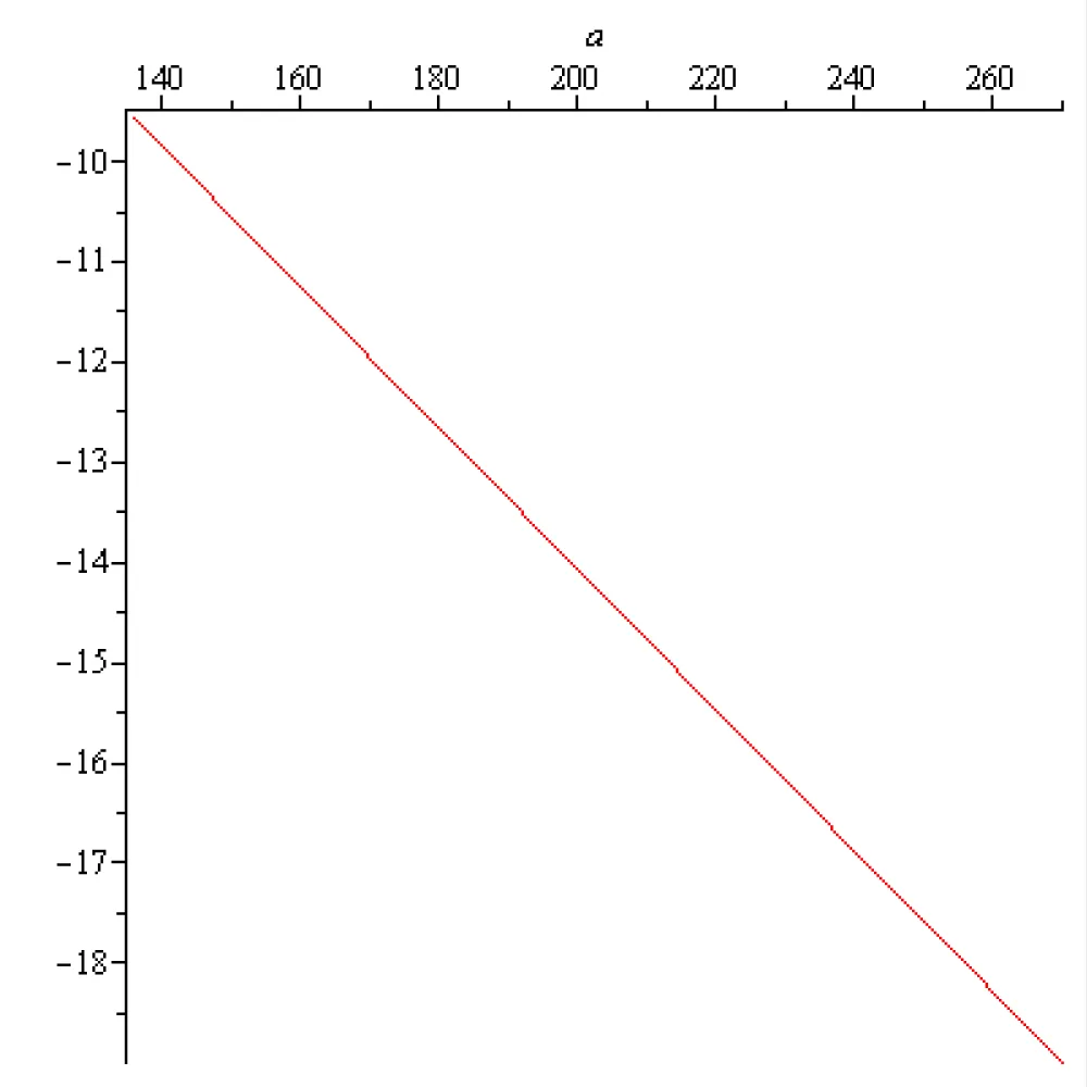
Figure 2.9: T versus a, for .
The sign minus physical meaning in this context is negative feedback (self-inhibition). It is related to instability. If T is negative, the rest state is unstable i.e., the rosehip cell voltage is no longer an energy minimum. The cell state tends to "run away" from the current state. For the initial state x0 = -70 × 10-3[V] and for two membrane ‘capacities a = 136[s]-1 and a = 270[s]-1 this "run away" dynamics is represented, with red and green colors respectively on the next Figure 2.10, 2.11 and 2.12:
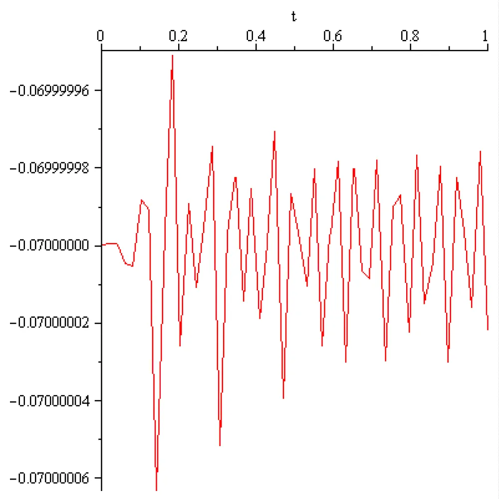
Figure 2.10: T = −9.566724239.
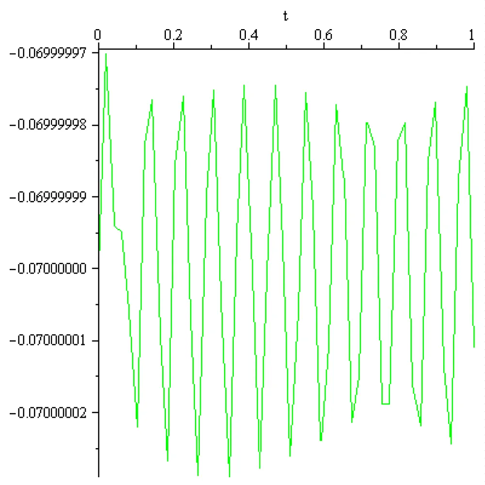
Figure 2.11: T = −18.99276136.
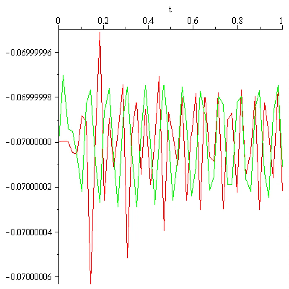
Figure 2.12: T = -9.566724239, T = -18.9927613.
-for the so called ‘Tanh’ input-output function, ; T ∈ [136.2220610, 270.4408564] and T varies according to the next Figure 2.13.
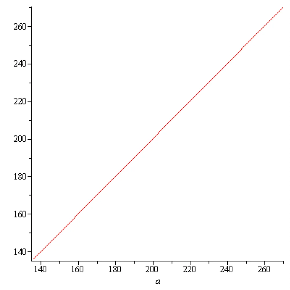
Figure 2.13: T versus a for .
The physical meaning of the plus sign in this context is positive feedback (self-excitation). It is related to stability. If T is positive, the rest state is stable i.e., the rosehip cell voltage is an energy minimum. If the neuron is in a current state, it tends to "reinforce" that state. For the initial state x0 = -70 × 10-3[V] and for two membrane ‘capacities’ a = 136[S]-1 and a = 270[S]-1 this dynamics is represented, with red and green colors respectively on the next Figure 2.14, 2.15 and 2.16:
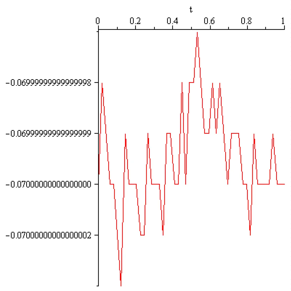
Figure 2.14: T = 136.2220610.
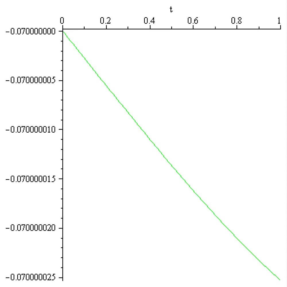
Figure 2.15: T = 270.4408564.
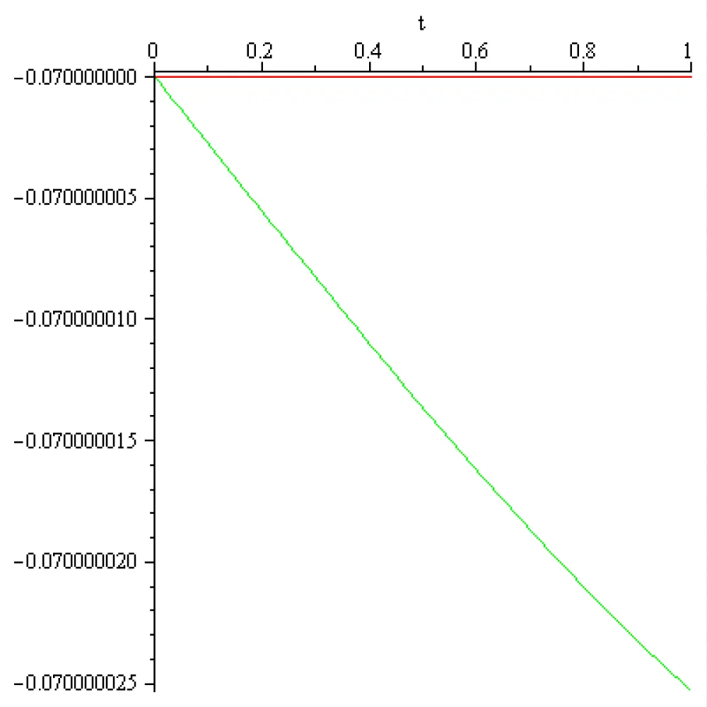
Figure 2.16: T = 136.2220610, T = 270.4408564.
-for the so called ‘Linear’ input-output function g(x) = x, T ∈ [136.0000000, 270.0000000] and T varies according to the next Figure 2.17.
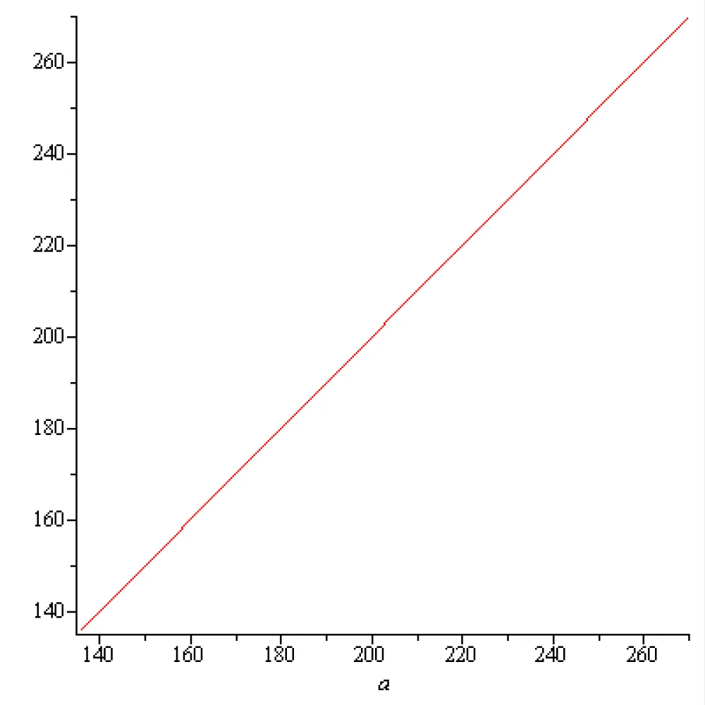
Figure 2.17: T versus a, for g(x) = x.
The physical meaning of the plus sign in this context is positive feedback (self-excitation). It is related to stability. If T is positive, the rest state is stable i.e., the rosehip cell voltage is an energy minimum. If the neuron is in a current state, it tends to "reinforce" that state. If the neuron is in a current state, it tends to "reinforce" that state. For the initial state x0 = -70 × 10-3[V] and for two membrane ‘capacities’ a = 136[S]-1 and a = 270[S]-1 this "reinforce" dynamics are represented, with red and green colors respectively on the next Figure 2.18, 2.19 and 2.20:
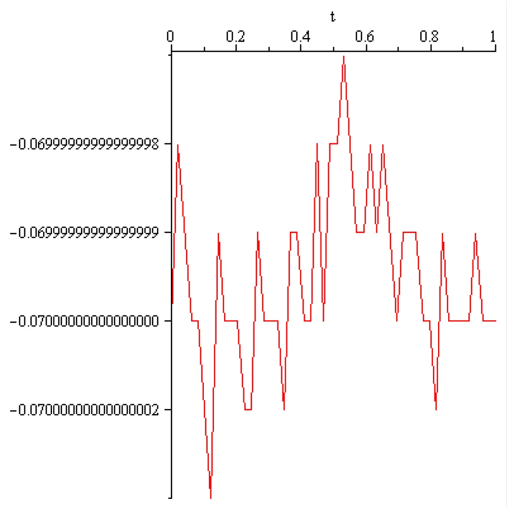
Figure 2.18: T = 136.
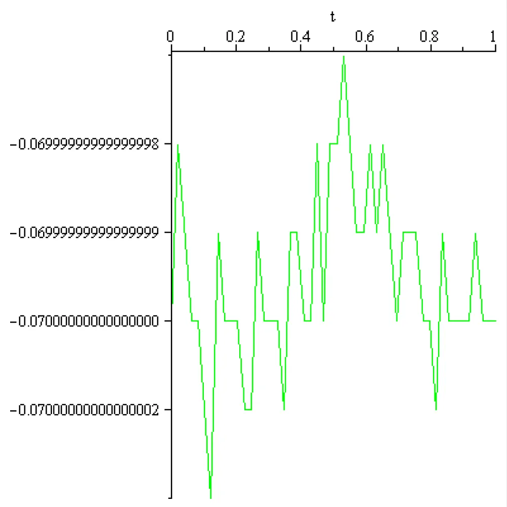
Figure 2.19: T = 270.
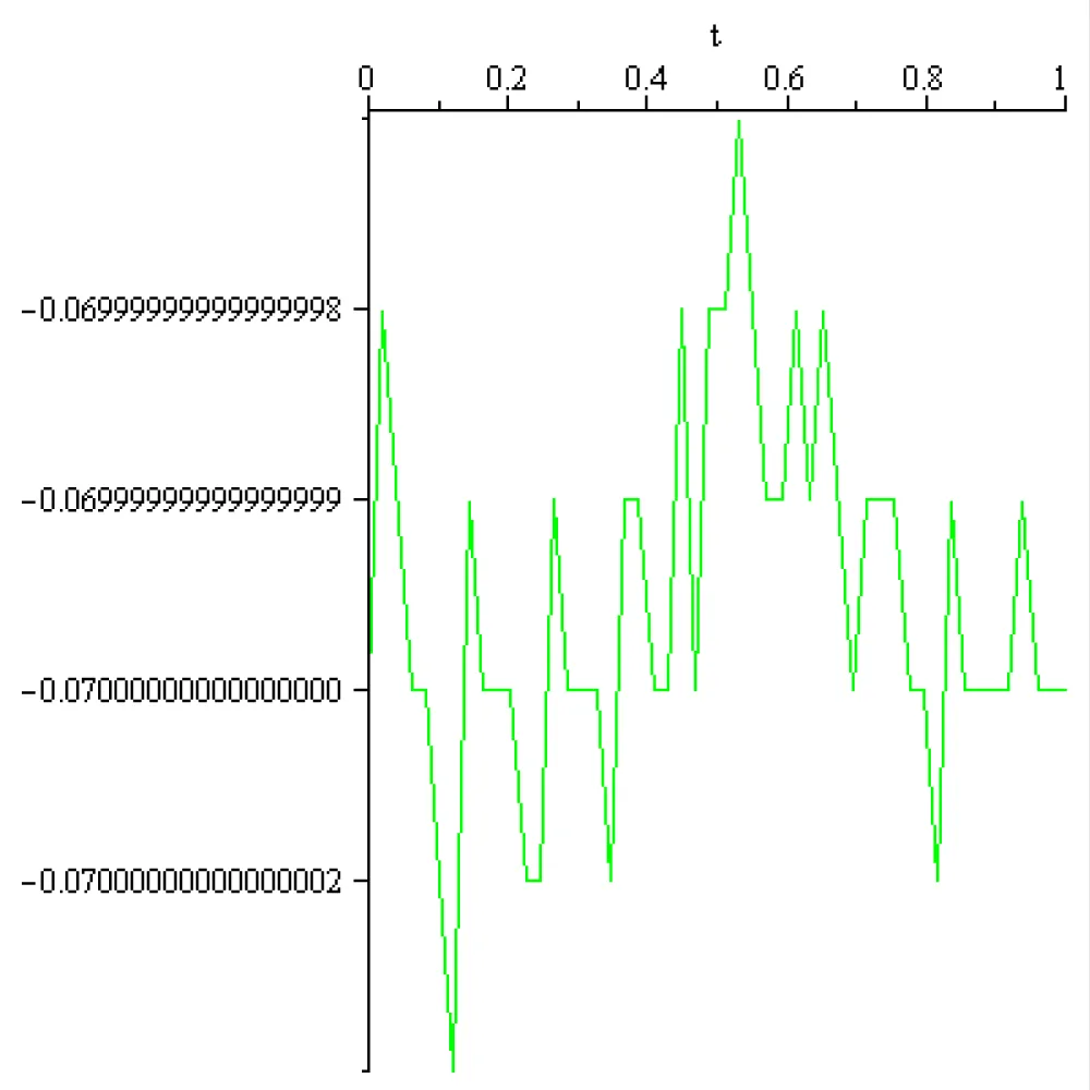
Figure 2.20: T = 136, T = 270.
-for the so called ‘Leaky ReLu’ input-output function g(x) = max (0.1 * x, x), T ∈ [136.0000000, 270.0000000], and T varies according to the next Figure 2.21.
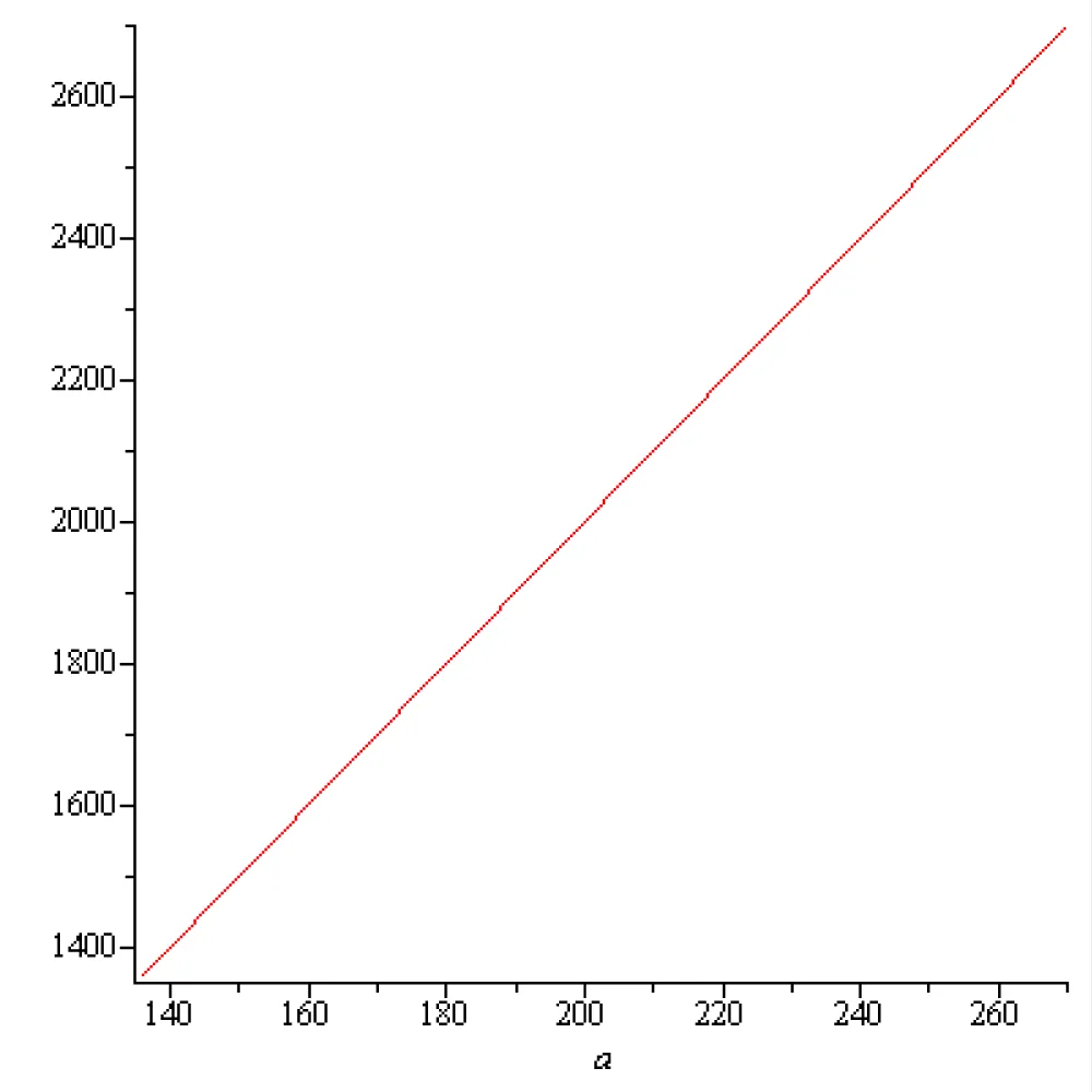
Figure 2.21: T versus a, for g(x) = max (0.1*x, x).
The physical meaning of the plus sign in this context is positive feedback (self-excitation). It is related to stability. If T is positive, the rest state is stable i.e., the rosehip cell voltage is an energy minimum. If the neuron is in a current state, it tends to "reinforce" that state. For the initial state x0 = -70 × 10-3[V] and for two membrane ‘capacities’ a = 136[S]-1 and a = 270[S]-1 this "reinforce" dynamics are represented, with red and green colors respectively on the next Figure 2.22, 2.23 and 2.24:
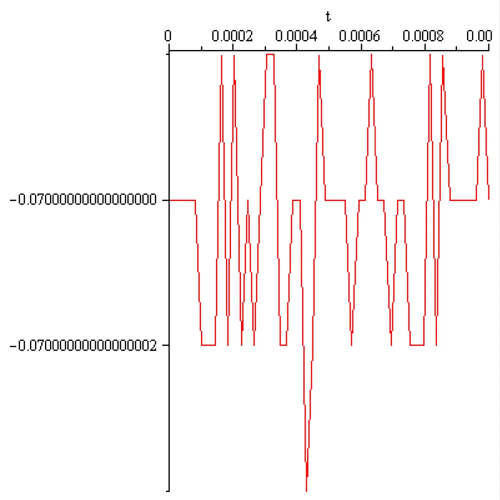
Figure 2.22: T = 1360.000000.
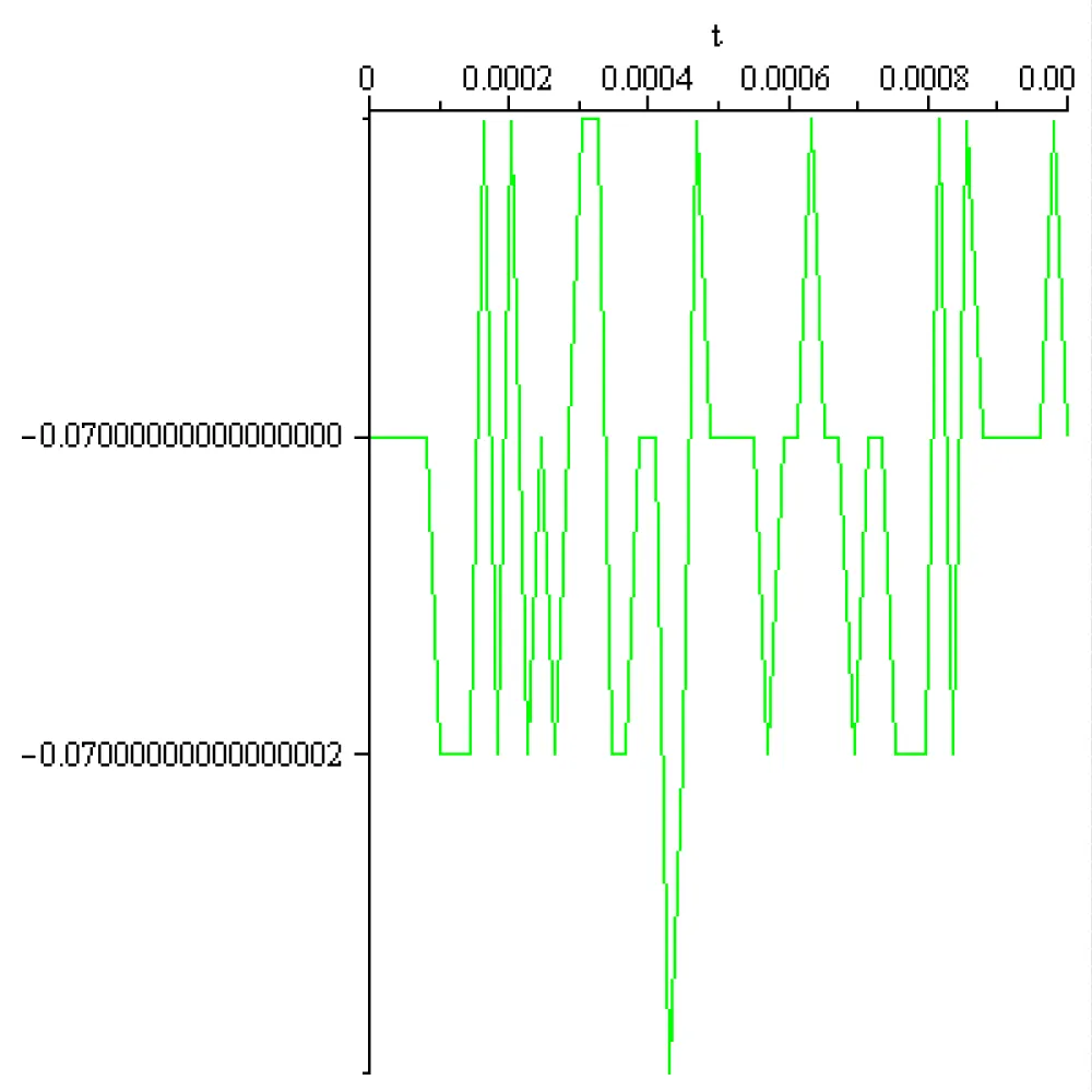
Figure 2.23: T = 2700.000000.
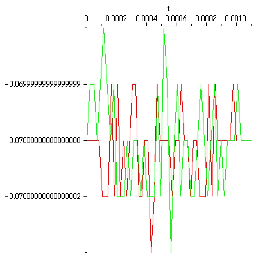
Figure 2.24: T = 1360.000000, T = 2700.000000.
-for the so called ‘Swish’ input-output function , T ∈ [281.8611126, 559.5772089], and T varies according to the next Figure 2.25.
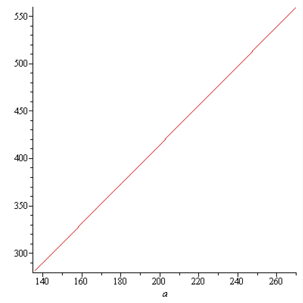
Figure 2.25: T versus a, for .
The physical meaning of the plus sign in this context is positive feedback (self-excitation). It is related to stability. If T is positive, the rest state is stable i.e., the rosehip cell voltage is an energy minimum. If the neuron is in a current state, it tends to "reinforce" that state. For the initial state x0 = -70 × 10-3[V] and for two membrane ‘capacities’ a = 136[S]-1 and a = 270[S]-1 this "reinforce" dynamics is represented, with red and green colors respectively on the next Figure 2.26, 2.27 and 2.28:
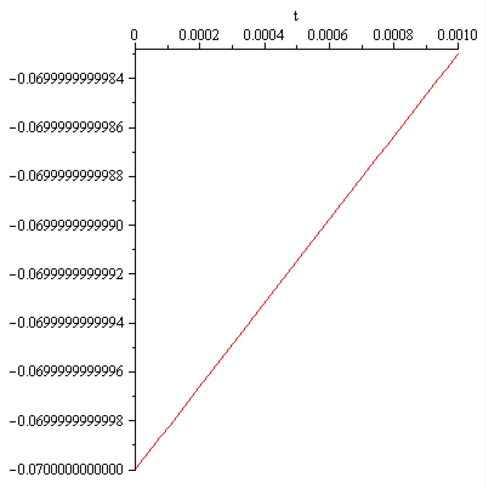
Figure 2.26: T = 281.8611126.
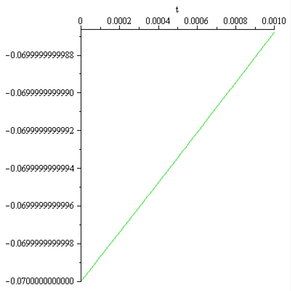
Figure 2.27: T = 559.5772089.
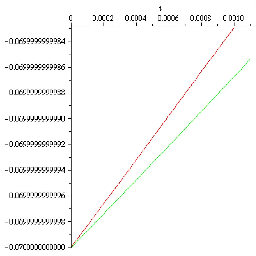
Figure 2.28: T = 281.8611126, T = 559.5772089.
-for the so called ‘ELU’ input-output function for x ≤ 0 and x for x > 0, T ∈ [,], and T varies according to the next Figure 2.29.
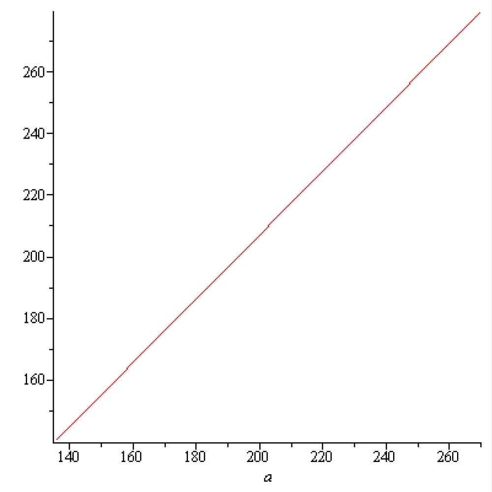
Figure 2.29: T versus a, for g(x) = 1 × (ex - 1) for × ≤ 0 and for x > 0.
The physical meaning of the plus sign in this context is positive feedback (self-excitation). It is related to stability. If T is positive, the rest state is stable i.e. the rosehip cell voltage is an energy minimum. If the neuron is in a current state, it tends to "reinforce" that state. For the initial state x0 = -70 × 10-3[V] and for two membrane ‘capacities’ a = 136[S]-1 and a = 270[S]-1 this "reinforce" dynamics is represented, with red and green colors respectively on the next Figure 2.30, 2.31 and 2.32:
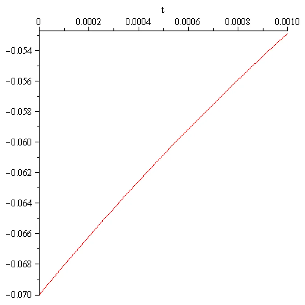
Figure 2.30: T = 140.8155288.
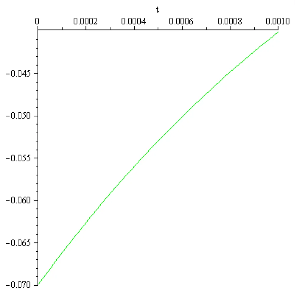
Figure 2.31: T = 279.5602409.
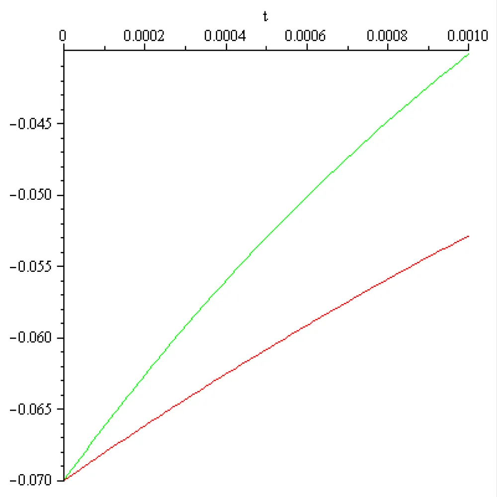
Figure 2.32: T = 140.8155288, T = 279.5602409.
-for the so called ‘GELU’ input-output function , [305.4596008, 606.4271486], and T varies according to the next Figure 2.33.
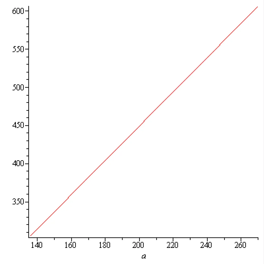
Figure 2.33: T versus a, for .
The physical meaning of the plus sign in this context is positive feedback (self-excitation). It is related to stability. If T is positive, the rest state is stable i.e., the rosehip cell voltage is an energy minimum. If the neuron is in a current state, it tends to "reinforce" that state. For the initial state x0 = -70 × 10-3[V] and for two membrane ‘capacities’ a = 136[S]-1 and a = 270[S]-1 this dynamics is represented, with red and green colors respectively on the next Figure 2.34, 2.35 and 2.36:
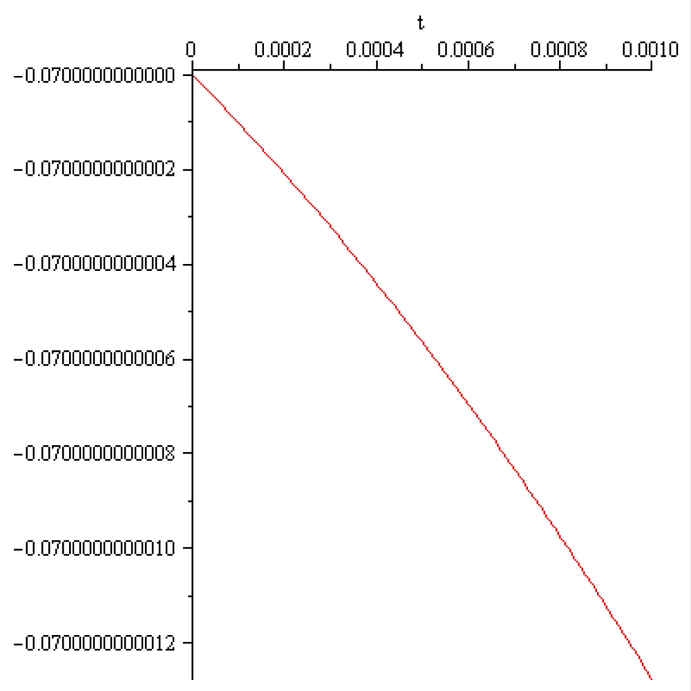
Figure 2.34: T = 305.4596008.
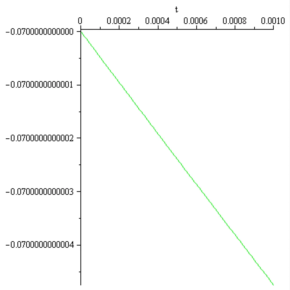
Figure 2.35: T = 606.4271486.
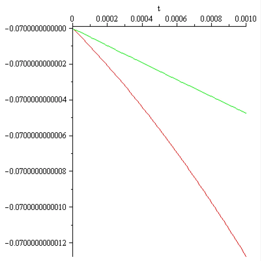
Figure 2.36: T = 305.4596008, T = 606.4271486.
The conclusions, obtained by computation, in this section can be summarized as follows:
-formula is an explicit functional relationship between the transfer co-efficient T the ‘membrane capacity a ‘and the input-output function value at the rest voltage -70 × 10-3[V].
- for the input-output functions: ‘Re LU’, ‘Dying Re LU’ and ‘Binary Step Function’ formula has no sense, so it is not appropriate for the determination of the transfer co-efficient T. (no feed-back).
-for the input-output functions: ‘Sigmoid/Logistic’, ‘Sigmoid*(1-Sigmoid)’, ‘Tanh derivative’, the transfer co-efficient T is negative, linear decreasing as function of the cell membrane capacity. If T is negative, then the feedback is negative (self- inhibition) the rest state is unstable i.e., the rosehip cell voltage is no longer an energy minimum. The cell state tends to "run away" from the current state.
-the dynamics of the rest state in case of ‘Sigmoid/Logistic’, ‘Sigmoid*(1-Sigmoid)’, ‘Tanh-derivative’, ‘Linear’, input-output activation functions, is oscillatory.
-in the case of ‘Tanh’, ‘Leaky Re Lu’ ‘Swish’, ‘ELU’, ‘GELU’ input-output activation functions the dynamics of the rest state is more specific. Namely:
-for ‘Tanh’: if a = 136[S]-1 then the rest voltage oscillate and if a = 270[S]-1 then the rest voltage decreases.
-for ‘Leaky Re Lu’:
if a = 136[S]-1 and 270[S]-1 then the rest voltage decreases
-for ‘Swish’ input-output function if a = 136[S]-1 and a = 270[S]-1 then the rest voltage increases
-for ‘ELU’ input-output function if a = 136[S]-1 and 270[S]-1 then the rest voltage increases
-for ‘GELU’ input-output function if a = 136[S]-1 and 270[S]-1 then the rest voltage decreases
3. Computed dynamics in the first stage (rest potential of -0.07[V] transfer into threshold potential of -0.055[V]) of the action potential for different membrane capacities and different input-output activation functions. External input values computed in the case of a single rosehip nervous cell, according to the Hopfield artificial neural network model
The rest potential is the difference in electrical charge (voltage) between the inside and outside of a rosehip nervous cell when it is not stimulated. It is a state of polarization, with the inside negative relative to the outside, usually -70 [mV], maintained by ion pumps and the selective permeability of the membrane (Figure 3.1, 3.2 and 3.3).
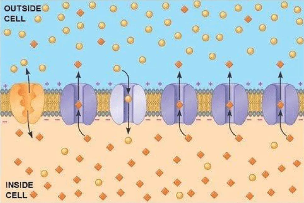
Figure 3.1: Rosehip nervous cell membrane.
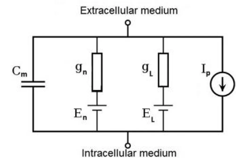
Figure 3.2: Electrical circuit model of a biological nervous cell membrane in the Hodgkin-Huxley model.
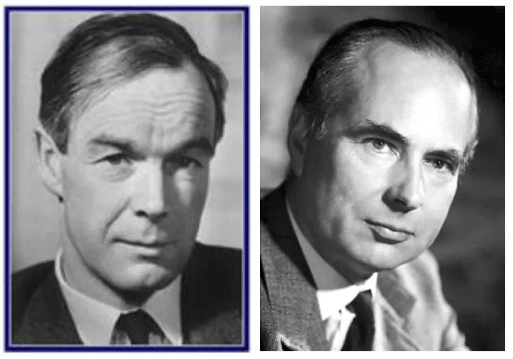
Figure 3.3: Alan Hodgkin and Andrew Huxley.
The Nobel Prize in Physiology or Medicine 1963 was awarded jointly to Sir John Carew Eccles, Alan Lloyd Hodgkin and Andrew Fielding Huxley for their discoveries concerning the ionic mechanisms involved in excitation and inhibition in the peripheral and central portions of the nerve cell membrane [4]. The typical Hodgkin-Huxley model treats each component of an excitable cell as an electrical element (as shown in the Figure 3.2). The lipid bilayer is represented as a capacitance (Cm). Voltage-gated ion channels are represented by electrical conductances (gn, where n is the specific ion channel) that depend on both voltage and time. Leak channels are represented by linear conductances (gL). The electrochemical gradients driving the flow of ions are represented by voltage sources (En) whose voltages are determined by the ratio of the intra- and extracellular concentrations of the ionic species of interest. Finally, ion pumps are represented by current sources (Ip). The membrane potential is denoted by Vm. Mathematically, the current flowing into the capacitance of the lipid bilayer is written as
(3.1)
and the current through a given ion channel is the product of that channel's conductance and the driving potential for the specific ion
(3.2)
Where Vi is the reversal potential of the specific ion channel. Thus, for a cell with sodium and potassium channels, the total current through the membrane is given by:
(3.3)
Using a series of voltage clamp experiments and by varying extracellular sodium and potassium concentrations, Hodgkin and Huxley developed a model in which the properties of an excitable cell are described by a set of four ordinary differential equations. Together with the equation for the total current mentioned above, these are:
(3.4)
Where I is the current per unit area and αi and βi are rate constants for the i-th ion channel, which depend on voltage but not time. is the maximal value of the conductance. n, m, and h are dimensionless probabilities between 0 and 1 that are associated with potassium channel subunit activation, sodium channel subunit activation, and sodium channel subunit inactivation, respectively.
For instance, given that potassium channels in squid giant axon are made up of four subunits which all need to be in the open state for the channel to allow the passage of potassium ions, the n needs to be raised to the fourth power. For p = (n, m, h), αp and βp take the form
(3.5)
(3.6)
are the steady state values for activation and inactivation, respectively, and are usually represented by Boltzmann equations as functions of Vm.
This model, conceived for one biological nervous cell, was extended for a network of biological nervous cells [5]. Due to the discrepancy between the computed and measured data, besides the integer order derivatives, the temporal fractional order derivative was introduced in the model [5]. The consequence was that the model became nonobjective [6].
Comparing the mathematical description defined by equations (3.4) with that defined by equations (2.1), we note that in the case of description (2.1) the consequences of opening and closing the gates must be described by changing the values of the external input current in (2.1).
The action potential is a rapid, temporary change in the rosehip membrane potential, whereby the inside becomes positive relative to the outside. First the rosehip nervous cell receives external input, which open the Na+ sodium channels. If the Na+ influx is large enough to raise the membrane potential from -70 [mV] to about -55 [mV], the threshold value, the "event" is triggered. Once the threshold is reached, the voltage-gated sodium channels open massively. Na+ ions rush into the cell, and the interior suddenly becomes positive up to +30 [mV] or +40 [mV].
For a rosehip nervous cell to fire an action potential, an incoming current must cause the membrane potential to depolarize from its resting potential around -70 [mV] to the threshold potential around -55[mV].
There is no single specific value for an input current that applies to all nervous cells; the required current varies depending on the neuron's type, size, and the desired outcome, but it is typically measured in pico-amperes or nano- amperes.
According to the Hopfield model the rosehip cell voltage dynamics presented above is governed by the solution of the differential equation:
(3.7)
corresponding to the initial value
x(0) = -0.07. (3.8)
Solving the initial value problem (3.7) numerically, (3.8) for a = 136[s]-1 and 270[s]-1, and T computed in the section 2 it turns that for I of order 10-12, 10-9[A] during the first 10[s] the voltage continues to oscillate around the rest potential. For the sigmoid input output activation function these oscillations are represented on the next Figure 3.4 and 3.5.
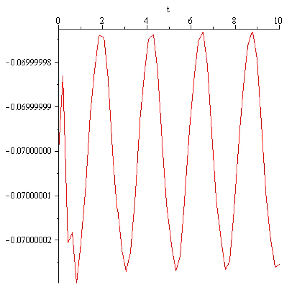
Figure 3.4: a = 136[s]-1, 1 = 10-9 [A], 10[s].
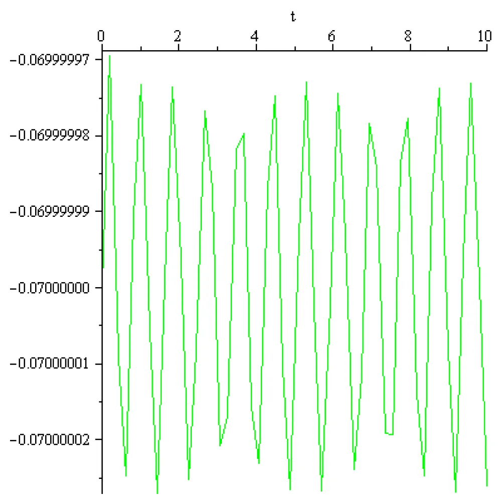
Figure 3.5: a = 270[s]-1, 1 = 10-9 [A], 10[s].
The above computational result and the lack of more detailed experimental data make us to make computational trials by increasing step by step the value of the external input I for obtain more realistic values for time frame and evolution towards the threshold potential. Observing that increasing I the time frame decreases we have fixed the time frame to the value of 0.15[s] and we have obtained by computation that in case of the sigmoid input-output function, the external input I for the activation potential (increase of -70[V] to -55[[V]) has to be taken: I = 2.13[A] for a = 136[s]-1 and I = 4.2[A] for a = 270[s]-1. The results of this computation is presented on the next Figure 3.6 and 3.7: -for g(x) Sigmoid
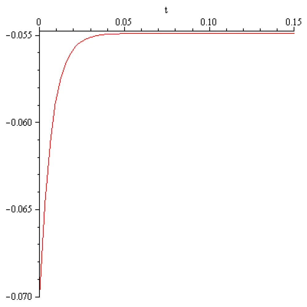
Figure 3.6: a = 136[s]-1, 1 = 2.13 [A], 0.15.
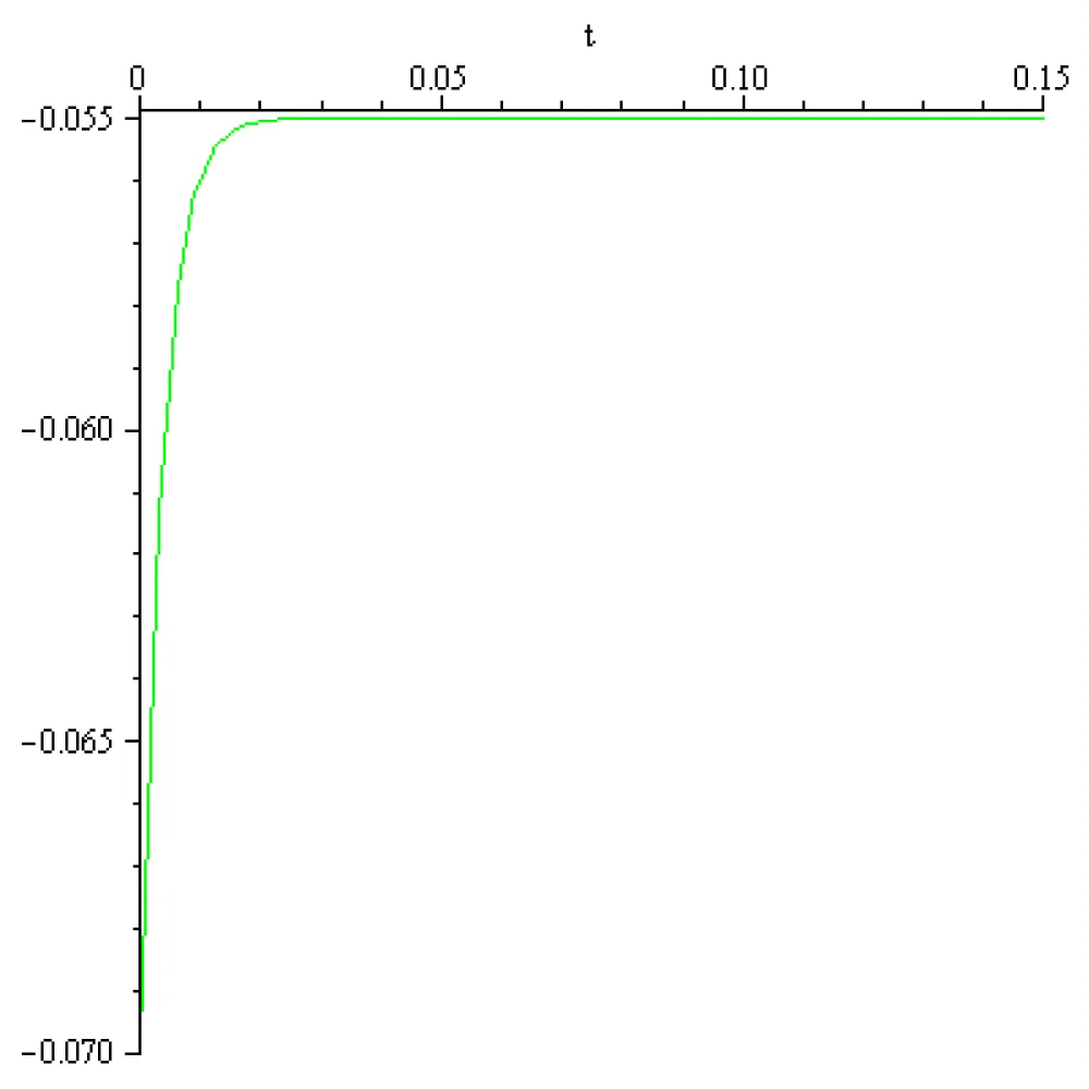
Figure 3.7: a = 270[s]-1, 1 = 4.2 [A], 0.15 [s].
The magnitude of the input currents obtained in these calculations differs extremely much from those discussed in literature (order of magnitude nano or pico amperes). Therefore, equation (3.7) doesn’t mirror correctly the reality. The ‘explanation’ of this discrepancy could be the Curie-von Sweidler law appearing in dielectric (i.e., in the double lipid layer of the cell membrane). Curie-von Schweidler law: refers to the response of dielectric material to the step input of a Direct Current (DC) voltage first observed by Jacques Curie [7,8] and Egon Ritter von Schweidler [9] The Curie current represents the response of a direct material to a step input DC votage. According to [7,8] the J.
Curie current intensity is given by
(3.9)
In [9] von Schweidler presents the main forms of abnormal behavior of dielectrics as follows.
If the terminals of a capacitor are connected to the poles of a current source with constant electromotive force, a current will appear in the conductors, the intensity of which decreases with time. For an ideal non-conducting dielectric, according to the general theory, the following differential equation applies to the "normal charging current":
(3.10)
Where C is the capacitance of the capacitor, L the self-inductance co-efficient, and R the resistance of the external circuit. Depending on the ratio of the numerical values of these three constants, the charging of the capacitor occurs either oscillatory or aperiodically. With a relatively small resistance of the external circuit, the current in each of the two traps decreases very rapidly, so that in practically realizable traps the normal charging current can be set to zero after times of the order of a small fraction of a second.
If the dielectric is not perfectly insulating, then a normal conduction current ‘a’ is superimposed on the normal charging current, ‘a’ is given by the formula
(3.11)
where λ is the specific conductance, K is the dielectric constant of the medium, C is the capacitance of the capacitor and E is the electromotive force of the current source (all quantities are considered to be measured in absolute electrostatic units).
In fact, as can be seen, in many dielectrics, besides the normal charging current and the normal conduction current, there is another "anomalous charging current" that overlaps, so that the entire current can be represented by:
(3.12)
Here, y1 is a function of time that asymptotically decreases to zero, but it is much more complex than the normal load current i1.
If the terminals of the capacitor are connected together after being maintained at a constant potential difference for a time interval δ, then two Open must be distinguished in terms of the laws of the discharge current:
a). The discharge current J2 corresponds to the normal discharge current i2, which is determined by an analogous integer differential equation, like the normal load current i1;
b). Analogous to the load, an “anomalous discharge current” y2 is superimposed, and y2 is again a function of it that decreases to zero with increasing time. The following relationship between y1 and y2is also valid:
(3.13)
That is, the total amount of electricity passing through a cross section of the conductor as a result of the abnormal discharge current is equal to the amount that was carried by the abnormal charge current during the charging period δ.
In case a), which is carried out especially with various poorly conductive liquids (Koller; Schweidler; Gadeke), the charging process proceeds as if the conductivity of the medium were undergoing temporal changes due to the passage of current.
In case b), the charging process is reversible; the medium behaves as if the conductivity corresponding to the time integral of the abnormal charging current . The amount of electricity absorbed is gradually released again during the discharge. This reversible process is usually referred to as the formation or pre-production of the "residue", and the integral as the "residual charge" formed during time δ.
In principle, the situation is less simple when the capacitor terminals are not held at constant potentials, but one of them is isolated; however, this form of residual phenomenon is historically the main one and this has led to the aforementioned name. If a capacitor is charged and then one of the two terminals is isolated, the potential difference V between the terminals, and therefore the so-called "dissipative charge" given by the product CV, decreases. This decrease occurs more rapidly than would correspond to the constant conduction current 'a'. Conversely, if the charged capacitor is discharged by temporarily connecting the terminals and only one terminal is isolated, a new charge of the same sign as the original gradually appears, increases to a maximum and then (due to the conduction of the dielectric) decreases asymptotically to zero. Regarding the laws that apply to the temporal evolution of residual phenomena and their dependence on other constraints, experimental investigations have led to the following results:
The anomalous charging current or residue formation current y1, at the terminals of a given capacitor with a given electromotive force, can be represented as a function of time by:
(3.14)
This formula can only be considered an approximation, because initially, we obtain for t = 0, γ1 = ∞. This means that equation (3.1) with ‘a’ constant is not appropriate for the description of real phenomenon. For more detail see [6,7].
For,and the time frame 0.15[s] the computed values of the external input for the other input-output functions are the followings.
-for g(x) Sigmoid*(1-Sigmoid)(Figures 3.8 and 3.9)
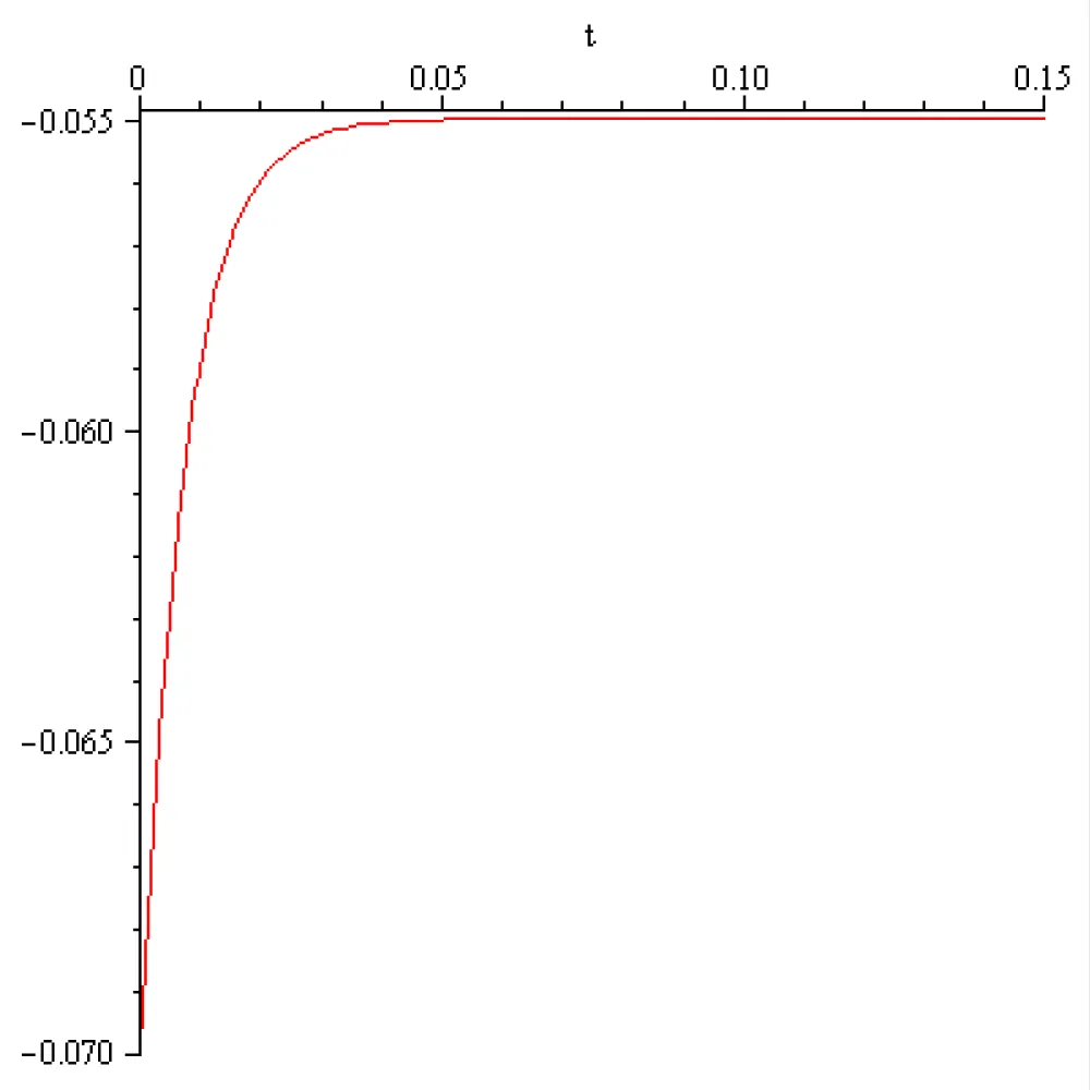
Figure 3.8: a = 136[s]-1, 1 = 2.05 [A], 0.15 [s].
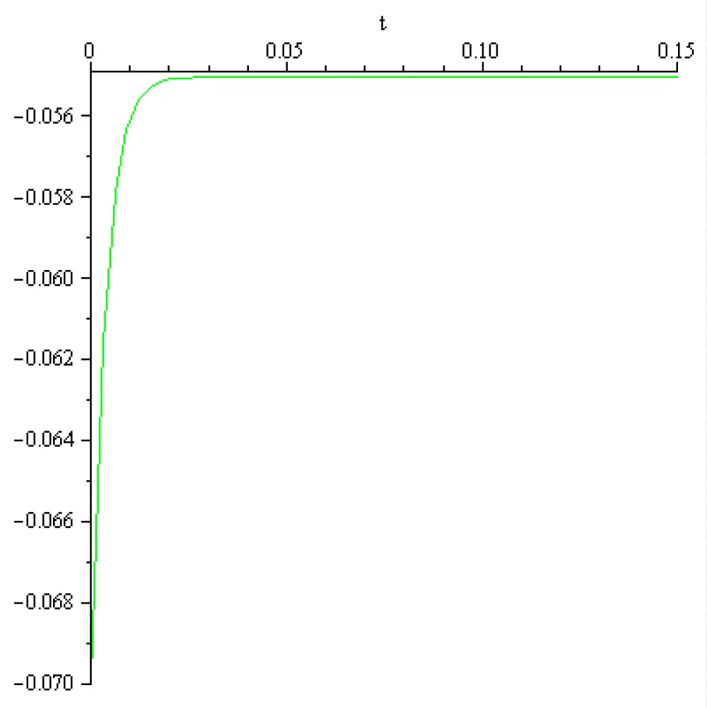
Figure 3.9: a = 270[s]-1, 1 = 4.05 [A], 0.15 [s].
-for g(x) Tanh-Derivative (Figure 3.10 and 3.11)
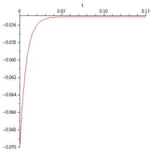
Figure 3.10: a = 136[s]-1, 1 = 2.05 [A], 0.15 [s].
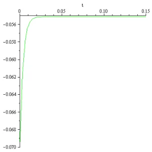
Figure 3.11: a = 270[s]-1, 1 = 4.05 [A], 0.15 [s].
-for g(x) Tanh (Figure 3.12 and 3.13)
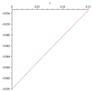
Figure 3.12: a = 136[s]-1, 1 = 0.1 [A], 0.15 [s].
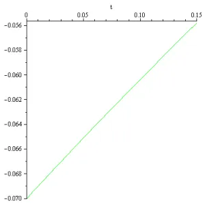
Figure 3.13: a = 270[s]-1, 1 = 0.1 [A], 0.15 [s].
-for g(x) Leaky ReLu (Figures 3.14 and 3.15)
-for g(x) Linear (Figure 3.14 and 3.15)
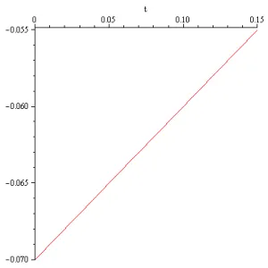
Figure 3.14: a = 136[s]-1, 1 = 0.1 [A], 0.15 [s].
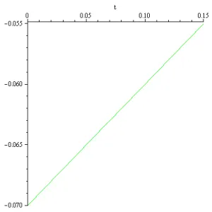
Figure 3.15: a = 270[s]-1, 1 = 0.1 [A], 0.15 [s].
-for g(x) Swish (Figures 3.16 and 3.17)
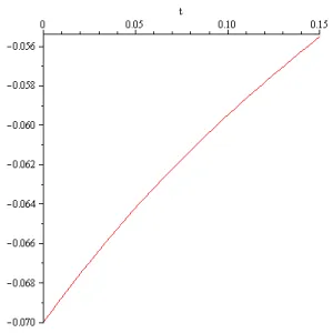
Figure 3.16: a = 136[s]-1, 1 = 0.13 [A], 0.15 [s].
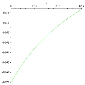
Figure 3.17: a = 270[s]-1, 1 = 0.1 7[A], 0.15 [s].
-forg (x) Elu (Figures 3.18 and 3.19)
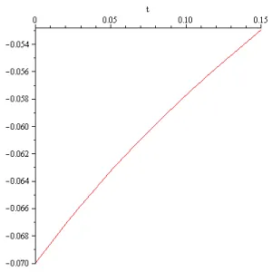
Figure 3.18: a = 136[s]-1, 1 = 0.15 [A], 0.15 [s].
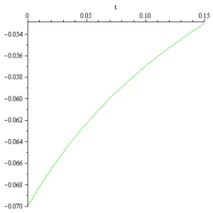
Figure 3.19: a = 270[s]-1, 1 = 0.19 [A], 0.15 [s].
-for g(x) Gelu (Figures 3.20 and 3.21)
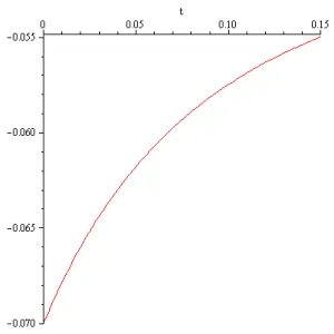
Figure 3.20: a = 136[s]-1, 1 = 0.235 [A], 0.15 [s].
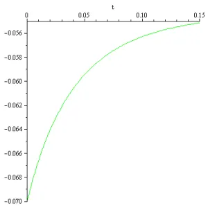
Figure 3.21: a = 270[s]-1, 1 = 0.4 [A], 0.15 [s].
At this stage the conclusions, obtained solving the initial value problem (3.7), (3.8), can be summarized as follows:
-for the input-output functions: sigmoid, sigmoid*(1-sigmoid), tanh-derivative the external input for transferring the rosehip nervous cell from the rest state of 0.07[V] into the threshold state 0.055 in a period of time of 0.15[s], is of order 100 [A].
-for the input output functions : tanh, linear,leaky relu, swish, elu, gelu the external input for transfer the rosehip nervous cell from the rest state of -0.07[V] into the threshold state -0.055 in a period of time of 0.15[s], is of order 10-1 [A].
- The magnitude of the input currents obtained in these calculations differs extremely much from those discussed in literature (order of magnitude nano or pico amperes). Therefore, the solution of the initial value problem (3.7), (3.8) doesn’t mirror the reality correctly. The ‘explanation’ of this discrepancy could be the Curie-von Schweidler law appearing in dielectric (i.e., in the double lipid layer of the cell membrane). Curie–von Schweidler law: refers to the response of a dielectric material to the step input of a Direct Current (DC) voltage, first observed by Jacques Curie [7,8] and Egon Ritter von Schweidler [9].
4. Computed dynamics in the second stage (threshold potential of -0.055[V] transfer into spike potential of +0.035[V]) of the action potential for different membrane capacities and different input-output activation functions. External input values computed in the case of a single rosehip nervous cell, according to the Hopfield artificial neural network model
In order to describe the phenomena mathematically: “Once the threshold is reached, the voltage-gated sodium channels open massively. Na+ ions rush into the cell, and the interior suddenly becomes positive up to +30 [mV] or +40 [mV]” we assume that:
- the effect of the massive opening of sodium channels and that of the Na+ ions rushing into the cell can be described by the increase of the exterior input in the cell, solving the initial value problem
(4.1)
x(0) = -0.055 (4.2)
Under the above hypothesis, the following computed results were obtained:
g(x) = Sigmoid/Logistic (Figures 4.1 and 4.2)
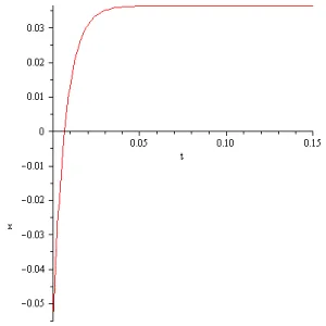
Figure 4.1: a = 136. I = 15[A], 0.15[s], sp.0.035[V].
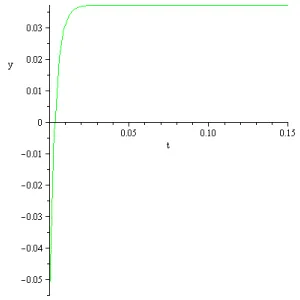
Figure 4.2: a = 270, I = 30[A], 0.15[s], sp. 0.035[V].
g(x) = Sigmoid*(1-Sigmoid) (Figures 4.3 and 4.4)
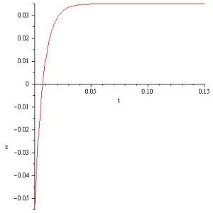
Figure 4.3: a = 136. I = 14.3[A]. 0.15[s], sp.0.035[V].
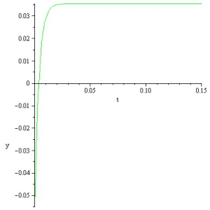
Figure 4.4: a = 270, I = 28.5[A], 0.15[s], sp.0.035[V].
g(x) Tanh-Derivative (Figures 4.5 and 4.6).
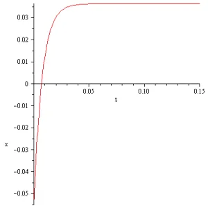
Figure 4.5: a = 136.I = 14.5[A]. 0.15[s], sp.0.035[V].
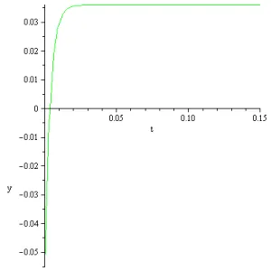
Figure 4.6: a = 270, I = 28.7[A], 0.15[s], sp.0.035[V].
g(x) = Tanh (Figures 4.7 and 4.8).
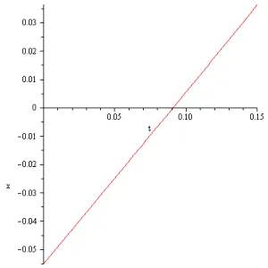
Figure 4.7: a = 136, I = 0.61[A]. 0.15[s], sp.0.035[V].
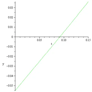
Figure 4.8: a = 270, I = 0.61[A], 0.15[s], sp.0.035[V].
g(x) = Linear (Figures 4.9 and 4.10).
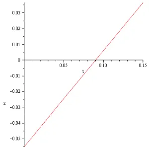
Figure 4.9: a = 136, I = 0.61[A]. 0.15[s], sp.0.035[V].
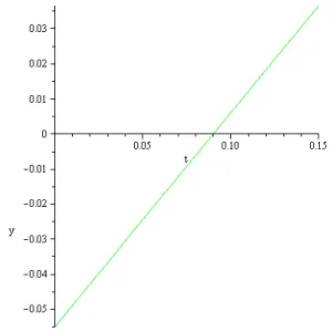
Figure 4.10: a = 270, I = 0.61[A], 0.15[s], sp.0.035[V].
g(x) = Leaky ReLu (Figures 4.11 and 4.12)
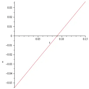
Figure 4.11: a = 136, I = 0.61[A], 0.15[s], sp.0.035[V].
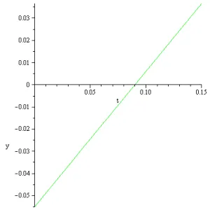
Figure 4.12: a = 270, I = 0.61[A], 0.15[s], sp.0.035[V].
g(x) = Swish (Figures 4.13 and 4.14)
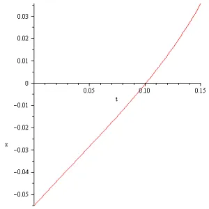
Figure 4.13: a = 136, I = 0.612[A]. 0.15[s], sp.0.035[V].
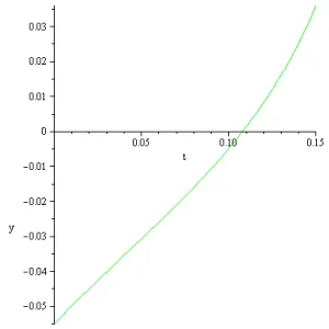
Figure 4.14: a = 270, I = 0.642[A], 0.15[s], sp.0.035[V].
g(x) = Elu (Figures 4.15 and 4.16)
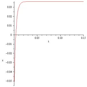
Figure 4.15: a = 136, I = 9.9[A], 0.15[s], sp.0.035[V].
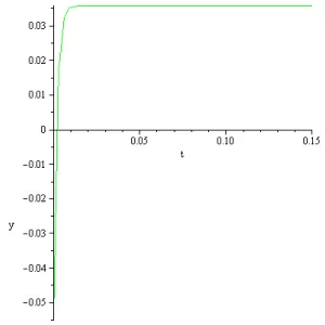
Figure 4.16: a = 270, I = 19.5[A], 0.15[s], sp.0.035[V].
g(x) = Gelu (Figures 4.17 and 4.18)
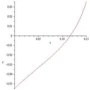
Figure 4.17: a = 136, I = 0.704[A], 0.15[s], sp.0.035[V].
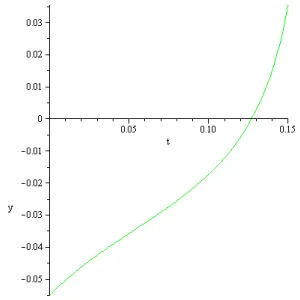
Figure 4.18: a = 270, I = 0.906[A], 0.15[s], sp.0.035[V].
- The above computation shows that in the case of the input-output functions sigmoid, sigmoid*(1-sigmoid), tanh-derivative, and elu, the magnitude of the input external impulse for transferring the threshold potential of -0.055[V] into the spike potential of +0.035[V]is of order 100[A]. In case of the input-output functions tanh, linear, leaky- relu, swish, and gelu, the magnitude of the input external impulse for transferring the threshold potential of -0.055[V] into the spike potential of +0.035[V] is of order 10-1[A].
- The magnitude of the input currents obtained in these calculations differs extremely much from those discussed in literature (order of magnitude nano or pico amperes). Therefore, the solution of the initial value problem (4.1), (4.2) doesn’t mirror the reality correctly. The ‘explanation’ of this discrepancy could be the Curie-von Schweidler law appearing in dielectric (i.e., in the double lipid layer of the cell membrane).
5. Computed dynamics in the third stage (spike potential of +0.035[V] transfer into the hyperpolarization potential of -0.077[V]) of the action potential for different membrane capacities and different input-output activation functions. External input values computed in the case of a single rosehip nervous cell, according to the Hopfield artificial neural network model
Concerning the process dynamics, as soon as the peak (+30 [mV] or +40 [mV]) of the action potential is reached, the cell must "reset" itself. Sodium channels close rapidly, potassium channels (K+) open, potassium ions leave the cell, carrying the positive charge out, and the interior of the cell becomes negative again. For a brief moment, the cell becomes a little more negative than normal -70 [mV] (hyperpolarization). At this stage, the rosehip neuron cannot fire another impulse, which ensures that the signal travels in only one direction (forward, down the axon) and does not return. The negative depolarization potential (or negative after potential) represents the phase after reaching the peak of the action potential, when the membrane potential remains for a short period, 40-50 [ms] less negative than the resting potential, but still negative, before returning completely to the initial state.
In order to describe mathematically, the process after the closure of sodium channels and opening of potassium channels, including hyperpolarization, we assume that the process is governed by the initial value problem:
(5.1)
x(0) = 0.035 (5.2)
and the exterior input, in the cell, was reduced during 0.15[s].
Solving the initial value problem (5.1), (5.2) for a = 136 and 270, g(x) presented and T computed in section 2, the following results concerning the rapid decrease of the negative depolarization of potential were obtained.
-for g(x) Sigmoid/Logistic (Figures 5.1 and 5.2)
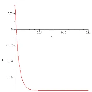
Figure 5.1: a = 136, I = -1[A], 0.15[s], hyp = -0.077[V].
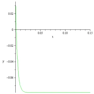
Figure 5.2: a = 270, I = -2.4[A], 0.15[s], hyp = -0.077[V].
-for g(x) Sigmoid*(1-Sigmoid) (Figures 5.3 and 5.4)
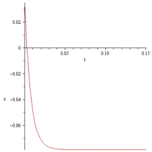
Figure 5.3: a = 136, I = -1.2[A], 0.15[s], hyp =-0.077[V].
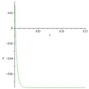
Figure 5.4: a = 270, I = -2.15[A], 0.15[s], hyp = -0.077[V].
-for g(x) Tanh-Derivative (Figures 5.5 and 5.6)
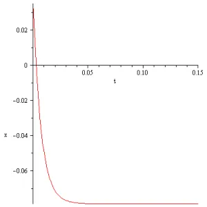
Figure 5.5: a = 136, I = -1.19[A], 0.15[s], hyp = -0.077[V].
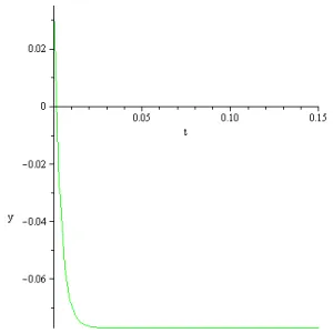
Figure 5.6: a = 270, I = -1.9[A], 0.15[s], hyp = -0.077[I].
-for g(x) Tanh (Figures 5.7 and 5.8)
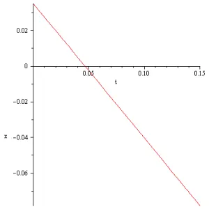
Figure 5.7: a = 136, I = -0.754[A], 0.15[s], hyp = -0.077[V].
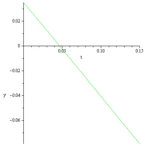
Figure 5.8: a = 270, I = -0.757[A], 0.15[s], hyp = -0.077[V].
-for g(x) Linear (Figures 5.9 and 5.10)
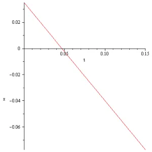
Figure 5.9: a = 36, I = -0.789[A], 0.15[s], hyp = -0.077[V].
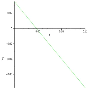
Figure 5.10: a = 270, I = -0.7489[A], 0.15[s], hyp = -0.077[V].
-for g(x) Leaky ReLu (Figures 5.11 and 5.12)
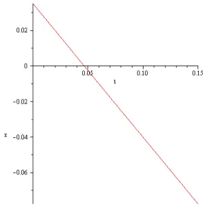
Figure 5.11: a = 136, I = -0.75[A], 0.15[s], hyp = -0.077[V].
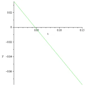
Figure 5.12: a = 270, I = -0.753[A], 0.15[s], hyp = -0.077[V].
-for g(x) Swish (Figures 5.13 and 5.14)
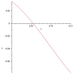
Figure 5.13: a = 136, I = -0.77[A], 0.15[s], hyp = -0.077[V].
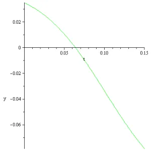
Figure 5.14: a = 270, I = -0.82[A], 0.15[s], hyp = -0.077[V].
-for g(x) Elu (Figures 5.15 and 5.16)
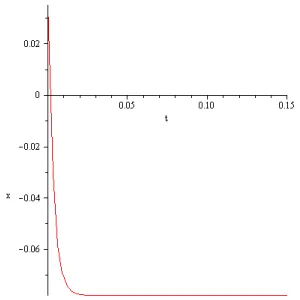
Figure 5.15: a = 136, I = -22[A], 0.15[s], hyp = -0.077[V].
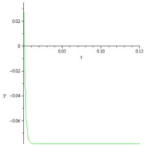
Figure 5.16: a = 270, I = -44[A], 0.15[s], hyp = -0.077[V].
-for g(x) Gelu (Figures 5.17 and 5.18)
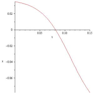
Figure 5.17: a = 136, I = -0.98[A], 0.15[s], hyp = -0.077[V].
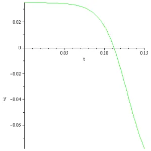
Figure 5.18: a = 270, I = -1.7472[A], 0.15[s], hyp = -0.077[V].
The global conclusion, obtained by solving the initial value problem (5.1), (5.2), can be summarized as follows:
-In the third stage, when the spike potential of +0.035[V] is transferred into the hyperpolarization potential of -0.077[V], the magnitude of the input currents obtained in these calculations differs extremely much from those discussed in literature (order of magnitude nano or pico amperes). Therefore, the solution of the initial value problem (5.1), (5.2) doesn’t mirror the reality correctly. The ‘explanation’ of this discrepancy could be the Curie-von Schweidler law appearing in dielectric (i.e., in the double lipid layer of the cell membrane).
6. Computed dynamics in the fourth stage (hyperpolarization potential of -0.077[V] transfer into the rest potential of -0.07[V]) of the action potential for different membrane capacities and different input-output activation functions. External input values computed in the case of a single rosehip nervous cell, according to the Hopfield artificial neural network model
In order to describe mathematically the return process of the rosehip hyperpolarization voltage of -0.077[V] to the rest voltage of -0.07[V] in the time frame of 0.04-0.05 [s], the following initial value problem was solved:
(6.1)
x(0) = -0.077 (6.2)
for a = 136 and 370, g(x) given and T computed in section 2. The following results concerning the voltage evolution from the value of -0.077 [V] to the resting voltage of -0.07[V] in 0.05 [s] were obtained.
-for g(x) Sigmoid/Logistic (Figures 6.1 and 6.2)
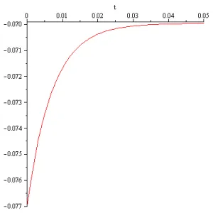
Figure 6.1: a = 136, I = -1[A], 0.15[s], hyp = -0.077[V].
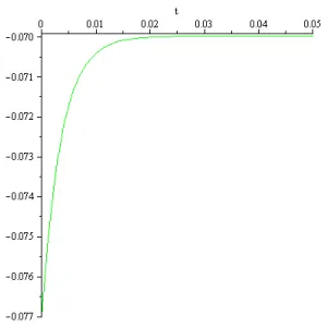
Figure 6.2: a = 270, I = -2.4[A], 0.15[s], hyp = -0.077[V].
-for g(x) Sigmoid*(1-Sigmoid) (Figures 6.3 and 6.4)
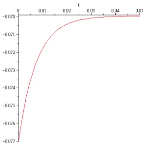
Figure 6.3: a = 136, I = -1.2[A], 0.15[s], hyp =-0.077[V].
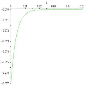
Figure 6.4: a = 270, I = -2.15[A], 0.15[s], hyp = -0.077[V].
-for g(x) Tanh-derivative (Figures 6.5 and 6.6)
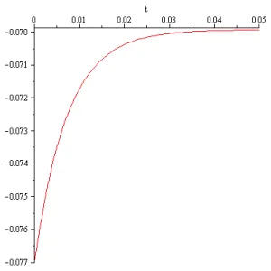
Figure 6.5: a = 136, I = -1.19[A], 0.15[s], hyp = -0.077[V].
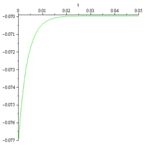
Figure 6.6: a = 270, I = -1.9[A], 0.15[s], hyp = -0.077[I].
-for g(x) Tanh (Figures 6.7 and 6.8)
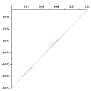
Figure 6.7: a = 136, I = -0.754[A], 0.15[s], hyp = -0.077[V].
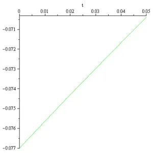
Figure 6.8: a = 270, I = -0.757[A], 0.15[s], hyp = -0.077[V].
-for g(x) Linear (Figures 6.9 and 6.10)
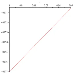
Figure 5.9: a = 36, I = -0.789[A], 0.15[s], hyp = -0.077[V].
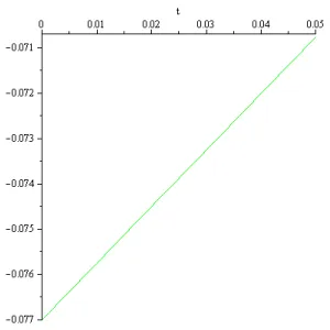
Figure 6.10: a = 270, I = -0.7489[A], 0.15[s], hyp = -0.077[V].
-for g(x) Leaky ReLu (Figures 6.11 and 6.12)
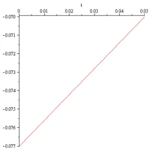
Figure 6.11: a = 136, I = -0.75[A], 0.15[s], hyp = -0.077[V].
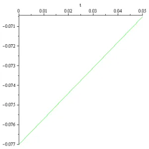
Figure 6.12: a = 270, I = -0.753[A], 0.15[s], hyp = -0.077[V].
-for g(x) Swish (Figures 6.13 and 6.14)

Figure 6: a = 136, I = -0.77[A], 0.15[s], hyp = -0.077[V].
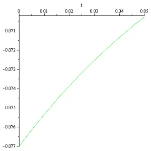
Figure 6.14: a = 270, I = -0.82[A], 0.15[s], hyp = -0.077[V].
-for g(x) Elu (Figures 6.15 and 6.16)
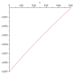
Figure 6.15: a = 136, I = -22[A], 0.15[s], hyp = -0.077[V].
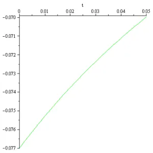
Figure 6.16: a = 270, I = -44[A], 0.15[s], hyp = -0.077[V].
for g(x) Gelu (Figures 6.17 and 6.18)
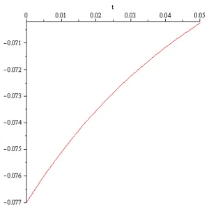
Figure 6.17: a = 136, I = -0.98[A], 0.15[s], hyp = -0.077[V].
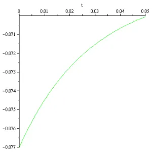
Figure 6.18: a = 270, I = -1.7472[A], 0.15[s], hyp = -0.077[V].
The global conclusion, obtained by solving the initial value problem (6.1), (6.2), can be summarized as follows:
-In the fourth stage, when the hyperpolarization potential of -0.077[V] is transferred into the rest potential of -0.07[V], the magnitude of the input currents obtained in these calculations differs extremely much from those discussed in literature (order of magnitude nano or pico amperes). Therefore, the solution of the initial value problem (6.1), (6.2) doesn’t mirror the reality correctly. The ‘explanation’ of this discrepancy could be the Curie-von Schweidler law appearing in dielectric (i.e., in the double lipid layer of the cell membrane).
7. Mirroring computed voltage oscillations in the case of a single rosehip nervous cell and dialogue between two rosehip cells, according to the Hopfield artificial neural network model
The computed results presented above provide a mirror of the oscillatory behavior of one rosehip nervous cell. Two computed successive oscillations in the case of the sigmoid input- output function are represented in the next Figure 7:
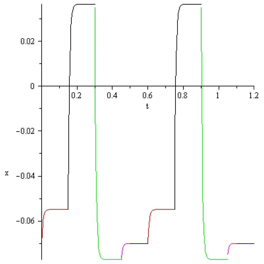
Figure 7: Two computed successive oscillations of the voltage state of one rosehip nervous cell.
Figure 7 shows that a complete oscillation has 5 stages.
The first stage marked in red color begins with the voltage increase from the rest voltage of -0.07[V] to the threshold voltage of -0.055[V]. This is due to an external input of +2.13[A] and lasts 0.15[s].
The second stage, marked in black color, is an increase in voltage from the threshold voltage of -0.055[V] to the spike voltage of +0.035[V]. This lasts 0.15[s] and is due to an external input of +15[A].
The third stage marked in green color is a decrease in voltage from +0.035[V] to -0.075[V]. This lasts 0.15[s] and is due to an external input of -1[A].
The fourth stage marked in magenta in the figure is an increase in voltage from -0.077 to -0.07[V]. This lasts 0.05[s] and is due to an external input of +0.006[A].
The fifth stage marked in blue in the figure is the rest voltage of -0.055[V]. It lasts for 0.005[s].
-In each stage, the magnitude of the input currents obtained in these calculations differs extremely much from those discussed in literature (order of magnitude nano or pico amperes). Therefore, Figure 7.1 doesn’t mirror the reality correctly. The ‘explanation’ of this discrepancy could be the Curie-von Schweidler law appearing in dielectric (i.e., in the double lipid layer of the cell membrane).
However, the results found allow us to compute in one artificial Hopfield neural network of two neurons, the dialogue of two rosehip cells. We will present dialogs of 0.15[s] and 0.05[s] in case of the sigmoid input- output function .
The system of differential equations that we use is:
(7.1)
Where: x[V] is the voltage of the first neuron, w[V] is the voltage of the second neuron; a = 136 [s]-1 is the ‘capacitance’ of the rosehip neuron membrane; T = -19.73027788 is the transfer coefficient corresponding to and a = 136[s]-1 In order to reveal the effect of the coefficients of the transfer matrix, we will consider two situations in each stage:
i). T12 = 0.1 and T21 = 0.1 ii). T12 = 0.1 and T21 = 1.
Ix[A] is the external input in the case of the first nervous cell and Iw[A] is the external input corresponding to the second nervous cell, depending on the stage of neurons. For simplicity, we will consider ‘dialogs’ when the first cell is in stage 1 and the second cell is in stages s1, s2, s3, s4.
i) First case: cell1 stage1, cell2 stage 1;
a). T12 = T21 = 0.1;
b). T12 = 0.1, T21 = 1; lasts 0.15[s].
The computed results are represented in the next Figures 7.1 and 7.2.
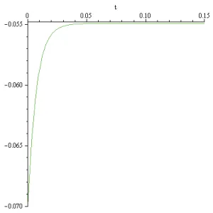
Figure 7.1: c1 s1, c2 s1, T12 = T21, voltage, c1 red, c2 green.
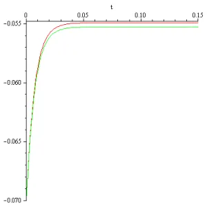
Figure 7.2: c1 s1, c2 s1, T12 = T21, voltage, c1 red, c2 green.
Figure 7.1 reveals a perfect similarity concerning the voltage dynamics in both cells due to the equality. T12 = T21. Computation shows that the shapes of the voltage graphics in the case of the system and individual cells are alike. At the end of 0.15[s] of the ‘dialog’ in the case of the system, the voltage of each of the cells is equal to:
x(t) = -0.054924823147208784[V],
w(t) = 0.054924823147208784[V]
On the other hand, the computed voltage at the end of the phase in the case of individual cells is -0.055[V]. Therefore, in this case, an increase of 1×10⁻³[V] appears in both cells.
Figure 7.2 reveals the effect of the inequality. T12 < T21 on the voltage dynamics in both cells. Computation shows that the shapes of the voltage graphics in the case of the system and individual cells are alike. At the end of the stage t = 0.15[s] in the case of the system, the voltage of each of the cells is equal too:
x(t) = -0.054925072179323838[V],
w(t) = -0.055275589201303106[V]
On the other hand, the computed voltage at the end of the phase in the case of individual cells is -0.055[V]. Therefore, in this case, an increase of 1×10⁻³[V] order appears in the first cell and a decrease of 2×10⁻⁴[V] order appears in cell 2.
ii) Second case: cell1, stage1; cell2, stage 2;
a). T12 = T21 = 0.1
b). T12 = 0.1, T21 =1; lasts 0.15[s] (Figures 7.3 and 7.4)
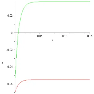
Figure 7.3: a = 136, I = -1.2[A], 0.15[s], hyp =-0.077[V].
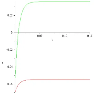
Figure 7.4: a = 270, I = -2.15[A], 0.15[s], hyp = -0.077[V].
Figure 7.3 reveals the effect of the stage of cell 2 on the voltage dynamics in both cells, although T12 = T21 = 0.1. Computation shows that the shapes of the voltage graphics in the case of the system and individual cells are alike. At the end of the stage t = 0.15[s] in the case of the system, the voltage of each of the cells is equal to:
x(t) = -0.0548600461167823434[V],
w(t) = 0.0363960892379317294[V]
On the other hand, the computed voltage at the end of the phase in the case of individual cells is -0.055[V] in cell 1 and +0.035[V] in cell 2. Therefore, in this case, an increase of
1×10⁻³[V] order appears in the first cell and an increase of
1×10⁻³[V] order appears in cell 2.
Figure 7.4 reveals the effect of the stage of cell 2 and the inequality. T12 < T21 on the voltage dynamics of both cells. Computation shows that the shapes of the voltage graphics in the case of the system and individual cells are alike. At the end of the stage t = 0.15[s] in the case of the system, the voltage of each of the cells is equal to:
x(t) = -0.0548602947527492626[V],
w(t) = 0.0360457451806459467[V]
On the other hand, the computed voltage at the end of the phase in the case of individual cells is -0.055[V] in cell 1 and +0.035[V] in cell 2. Therefore, in this case, at the end of the dialogue, an increase of 1×10⁻³[V] order appears in the first cell and an increase of 1×10⁻³[V] order appear in cell 2.
iii) Third case: cell1, stage1; cell2, stage 3;
a). T12 = T21 = 0.1;
b). T12 = 0.1, T21 = 1; lasts 0.15[s] (Figures 7.5 and 7.6)
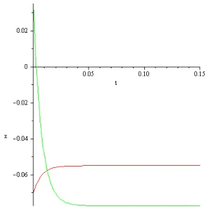
Figure 7.5: c1 s1, c2 s3, T12 = T21, voltage, c1 red, c2 green.
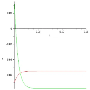
Figure 7.6: c1 s1, c2 s3, T12 = T21, voltage, c1 red, c2 green.
Figure 7.5 reveals the effect of the stage of cell 2 on the voltage dynamics in both cells, although T12 = T21 = 0.1. Computation shows that the shapes of the voltage graphics in the case of the system and individual cells are alike. At the end of the stage t = 0.15[s] in the case of the system, the voltage of each of the cells is equal to:
x(t) = -0.0549406048677065564[V],
w(t) = -0.0771349115385281392[V]
On the other hand, the computed voltage at the end of the phase in the case of individual cells is -0.055[V] in cell 1 and -0.077[V] in cell 2. Therefore, in this case, an increase of
1×10⁻³[V] order appears in the first cell and a decrease of
1×10⁻⁴[V] order appears in cell 2.
Figure 7.6 reveals the effect of the stage of cell 2 and the inequality. T12 < T21 on the voltage dynamics of both cells. Computation shows that the shapes of the voltage graphics in the case of the system and individual cells are alike. At the end of the stage t = 0.15[s] in the case of the system, the voltage of each of the cells is equal to:
x(t) = -0.0549408538170100130[V],
w(t) = -0.0774857842923780682[V]
On the other hand, the computed voltage at the end of the phase in the case of individual cells is -0.055[V] in cell 1 and -0.077[V] in cell 2. Therefore, in this case, at the end of the dialogue, an increase of 1×10⁻³[V] order appears in the first cell and a decrease of 1×10⁻⁴[V] order appears in cell 2.
iv) Fourth case: cell1, stage1; cell2, stage 4;
a). T12 = T21 = 0.1;
b). T12 = 0.1, T21 = 1; lasts 0.05[s] (Figures 7.7 and 7.8)
Figure 7.7 reveals the effect of the stage of the cell 2 on the voltage dynamics in both cells although T12 = T21 = 0.1. Computation shows that the shapes of the voltage graphics in the case of the system and individual cells are alike. At the end of the stage t = 0.05[s] in the case of the system, the voltage of each of the cells is equal to:
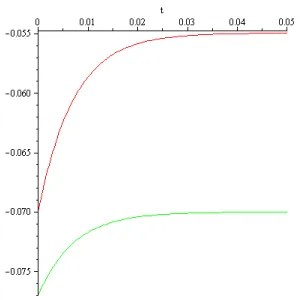
Figure 7.7: c1 s1, c2 s4, T12 = T21, voltage,c1 red, c2 green.
x(t) = -0.0549486597556062342[V],
w(t) = -0.0700025581813548958[V]
On the other hand, the computed voltage at the end of the phase in the case of individual cells is -0.055[V] in cell 1 and -0.07[V] in cell 2. Therefore, in this case, an increase of
1×10⁻³[V] order appears in the first cell and a decrease of
1×10⁻⁶ [V] order appears in cell 2.
Figure 7.8 reveals the effect of the stage of cell 2 and the inequality. T12 < T21 on the voltage dynamics of both cells. Computation shows that the shapes of the voltage graphics in the case of the system and individual cells are alike. At the end of the stage t = 0.05[s] in the case of the system, the voltage of each of the cells is equal to:
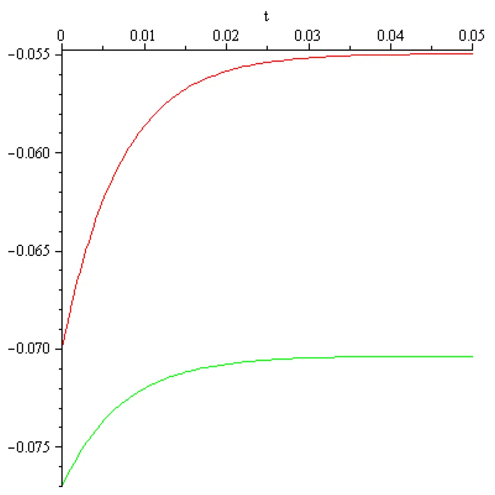
Figure 7.8: c1 s1, c2 s4, T12 = T21, voltage, c1 red, c2 green.
x(t) = -0.0549489084336642966[V],
w(t) = -0.070353681036605039[V]
On the other hand, the computed voltage at the end of the phase in the case of individual cells is -0.055[V] in cell 1 and -0.07[V] in cell 2. Therefore, in this case, at the end of the dialogue, an increase of 1×10⁻³[V] order appears in the first cell and a decrease of 1×10⁻⁴ [V] order appears in cell 2.
-One of the conclusions obtained in this section is that the voltage dynamics, reported empirically for the rosehip nervous cell, can be mirrored in the framework of the Hopfield artificial network. What is remarkable is that the spikes are not so sharp as in the case of the ECG.
A second conclusion is that a ‘dialog’ between two rosehip neuron cells can be mirrored.
This paper provides a mirroring of the voltage dynamics of a rosehip nervous cell in a continuous-time Hopfield artificial neural network. The global conclusion is that every stage of the voltage dynamics can be mirrored. Unfortunately, the magnitude of the input currents obtained in these calculations differs extremely much from those discussed in literature (order of magnitude nano or pico amperes). Therefore, the mirroring authenticity is questionable.
The ‘explanation’ of this discrepancy could be the Curie-von Schweidler law appearing in dielectric (i.e., in the double lipid layer of the cell membrane). Curie-von Schweidler law: refers to the response of a dielectric material to the step input of a Direct Current (DC) voltage, first observed by Jacques Curie [7,8] and Egon Ritter von Schweidler [9].
Authors contribution
The authors contributed equally to the realization of this work. All authors have read and agreed to the published version of the manuscript.
Founding
This research did not receive any specific grant from founding agencies in the public, commercial or not-for-profit sectors.
Data availability statement
The original contributions presented in the study are included in the article; further inquiries can be directed to the corresponding author.
- Mike M. Scientists Have Found a New Type of Brain Cell, and It Looks Like It's Unique to Humans. Science Alert. Retrieved 2018-09-01. Available from: https://www.sciencealert.com/rosehip-neuron-discovery-absent-in-mouse-models
- Boldog E, Bakken TE, Hodge RD, Novotny M, Aevermann BD, Baka J, et al. Transcriptomic and morphophysiological evidence for a specialized human cortical GABAergic cell type. Nat Neurosci. 2018 Sep;21(9):1185-1195. Available from: https://doi.org/10.1038/s41593-018-0205-2
- Balint S, Braescu L, Kaslik E. Regions of attraction and applications to control theory. Cambridge Scientific Publishers Ltd. 2008. Edited by S. Sivasundaram.
- Hodgkin AL, Huxley AF. A Quantitative Description of Membrane Current and Its Application to Conduction and Excitation in Nerve. J Physiol Lond. 1952;117(4): 500-544. Available from: https://doi.org/10.1113/jphysiol.1952.sp004764
- Weinberg SH. Membrane Capacitive Memory Alters Spiking in Neurons Described by the Fractional Order Hodgkin-Huxley Model” PloS ONE.2015;10(5):e0126629. Available from: https://doi.org/10.1371/journal.pone.0126629
- Balint AM, Balint S, Szabo R. Mathematical description of the ion transport across biological neuron membrane and in biological neuron networks, voltage propagation along neuron axons and dendrites, which use temporal classic Caputo or Riemann-Liouville fractional partial derivatives, is non-objective. MESA. 2021;12(4).p. 1057.
- Curie J. Recherches sur le pouvoir inducteur spécifique et sur la conductibility des corps cristallisés". Annales de Chimie et de Physique. 1889;17: 384–434.
- Curie J. Recherches sur la conductibilité des corps cristallisés". Annales de Chimie et de Physique. 1889;18: 203–269.
- Schweidler E, Physics, der Physik A. Studien über die Anomalien im Verhalten der Dielektrika (Studies on the anomalous behavior of dielectrics). 1907;329(14): 711–770. Available from: https://doi.org/10.1002/ANDP.19073291407
- Cojocaru AV, Balint S. Are power laws similar to constitutive laws? Can be incorporated in the same way in the existing equations, boundary conditions, initial conditions describing real world phenomena? Is this a way to avoid temporal fractional order derivatives? 2026;2: 1-31. Available from: https://doi.org/10.71448/tk202621