
More Information
Submitted: August 03, 2026 | Accepted: August 06, 2026 | Published: August 07, 2026
Citation: Kumar K. Thermal Analysis of Lead-Free Ceramics. Int J Phys Res Appl. 2026; 9(8): 261-264. Available from:
https://dx.doi.org/10.29328/journal.ijpra.1001164
DOI: 10.29328/journal.ijpra.1001164
Copyright license: © 2026 Kumar K. This is an open access article distributed under the Creative Commons Attribution License, which permits unrestricted use, distribution, and reproduction in any medium, provided the original work is properly cited.
Nomenclature: Electronic conductivity; Ionic polarization; Space charge; Ceramic constant

Thermal Analysis of Lead-Free Ceramics
Kanchan Kumar*
Assistant Professor, University Dept. of Physics, T. M. Bhagalpur University, Bhagalpur, India
*Address for Correspondence: Kanchan Kumar, Nygårdsvej 10, 2s., Nr.13, 2100, Østerbro, Copenhagen, Denmark, Email: [email protected]
Thermal analysis of lead-free ceramics is based on temperature variation leading to theoretical assessment anticipating the normal conductivity and a.c. conductivity of the material. It is also seen that the change in polarization includes electronic and ionic polarization. The effect of temperature on both electronic and ionic polarization is small at short domains. At high temperature, polarization increases due to the ionic and crystal imperfection mobility. The joint effect creates a pointed increase in the dielectric constant with an increase in temperature, which is correspondent to orientation of the dipole and space charge. The extension of the exponential function into a series expansion has been used to view the specific changes. The a.c. conductivity of the ceramic is theoretically calculated, inculcating at small domain of the Fermi level with photonic frequency. With the help of electronic charge, photonic frequency, and Boltzmann constant, a new ceramic constant σc is calculated, leading to the remarkable varying a. c. conductivity controlling the density. The virtual readings are set up to view the theoretical consequences that tend to explain the normal and a. c. conductivity of the material. The corresponding Graphical variation shifts to the crucial points of the inculcated plan.
Some of the ceramics have enormous potential and extraordinary features that make them to be used in many devices such as sensors, detectors, optical switches, actuators, radio-frequency filters, etc. Perovskite [1] ABO3-type Ferromaterials have fascinated the Researchers since several decades, targeting applications such as capacitors, Pizoelectric transducers, Pyroelectric detectors, and various micro-electronic devices due to their outstanding properties. It is found that mostly the materials are manufactured from compounds containing lead, such as PbTiO3, Pb(ZrTi)O3, Pb( ) etc. However, the lead-containing ceramics cause environmental pollution and generate instability of the constituent and electrical properties of the products. Moreover, it has been seen lead based gadgets are not recyclable. The Researchers sought a way to prepare lead-free ceramics replacing the existing Pb-based materials.
The materials lead free ceramics are to be fabricated using solid state Reaction Technique i.e., very effective and industrially preferable, with variation in temperature. It requires heating the precursors to a high temperature (about 1000oC). Since the material has no reaction at room temperature (25oC). The whole process [1] is executed in six successive steps: proper stoichiometry, drying and mixing followed by Wet mixing, calcinations, Grinding and Pelletization, sintering, and Electroding.
The normal conductivity of ceramics at Temperature T is given by
(1)
Where, Ea = Activation Energy, Kb is the Boltzmann constant.
The a.c. conductivity [2,3] of the ceramics at temperature T is given by
(2)
Where, e = electronic charge, ω = frequency, f0 = photonic frequency,
N(EF)= Fermi levels, α = localized wave function
From eqn. (1)
Neglecting the higher-order terms, we have…
(3)
Reduced Equation (4)
Where, A = neglecting 1; constant A = 1.73×𝟏𝟎𝟒 Kelvin.
This relation shows that normal conductivity is inversely proportional to Temperature, goes on decreasing with different values as given in Table 1.
| Table 1: The graph between temperature and conductivity | |||
| S.N. | Temperature( | T(K) | Conductivity |
| 1 | 1000 | 1273 | 0.785 x 10⁻³ |
| 2 | 1020 | 1293 | 0.773 x 10⁻³ |
| 3 | 1030 | 1303 | 0.767 x 10⁻³ |
| 4 | 1040 | 1313 | 0.761 x 10⁻³ |
| 5 | 1050 | 1323 | 0.755 x 10⁻³ |
| 6 | 1060 | 1333 | 0.750 x 10⁻³ |
| 7 | 1070 | 1343 | 0.744 x 10⁻³ |
| 8 | 1080 | 1353 | 0.739 x 10⁻³ |
Corresponding graph between temperature and conductivity is depicted as follows:
Figure 1: Temperature in Kelvin vs conductivity
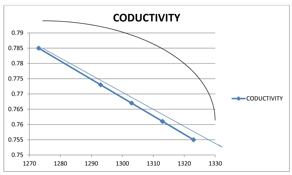
Figure 1: Temperature vs. conductivity.
The a.c. conductivity of the material is taken from Equation (2)
Considering other terms constant irrespective of the Temperature
(5)
Where,
since,
α = 1, and taking = 1 we calculate Ceramic constant σc = 3.56 electron volt
The virtual calculation with the different values of Temperature, a.c. conductivity is observed as below Table 2.
| Table 2: The graph between temperature and a.c. conductivity. | |||
| S.N. | Temperature(oC) | T(K) | a.c. conductivity = σc.T ´ 10-23(eV). |
| 1 | 1000 | 1273 | 4.531 |
| 2 | 1020 | 1293 | 4.603 |
| 3 | 1030 | 1303 | 4.638 |
| 4 | 1040 | 1313 | 4.674 |
| 5 | 1050 | 1323 | 4.709 |
| 6 | 1060 | 1333 | 4.745 |
| 7 | 1070 | 1343 | 4.781 |
| 8 | 1080 | 1353 | 4.816 |
The corresponding graph between temperature and a.c. conductivity is plotted as follows: Figure 2.
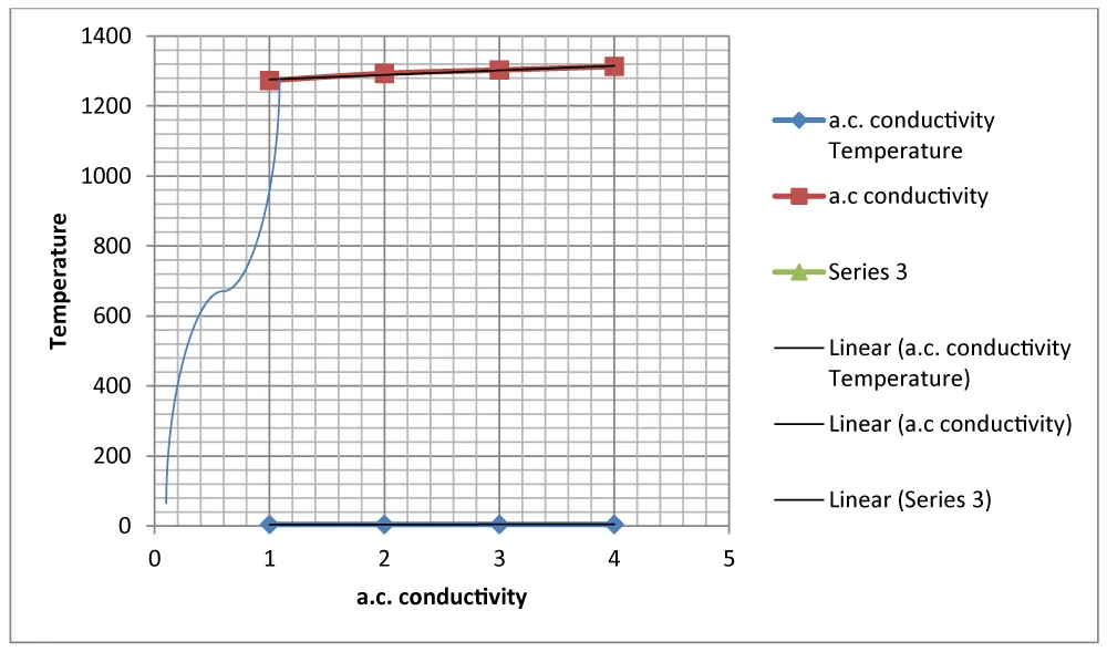
Figure 2: Temperature vs. a. c. conductivity.
The experimental graph of a. c. conductivity with respect to frequency and temperature is shown in Figure. 3 (a) and 3 (b):
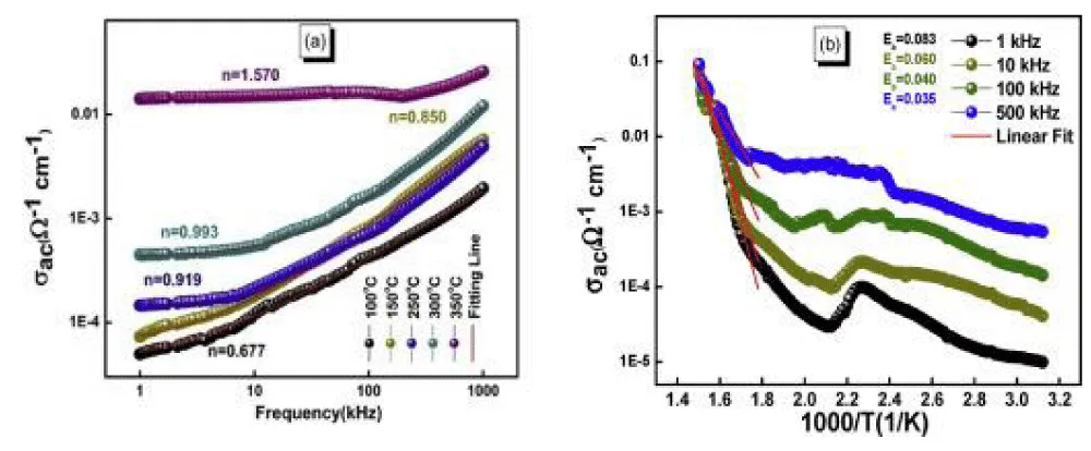
Figure 3: (a) Frequency vs. a.c. conductivity and (b) temperature vs. a.c. conductivity.
Frequency variation of total conductivity at different temperatures is discussed with the following data: Tables 3,4.
| Table 3: A graph between frequency, temperature and a.c. condutivity | |||
| S.N. | Frequency(f) | Temperature()(T) | σac |
| 1 | 10 | 50 | 10-11 |
| 2 | 101 | 100 | 10-9 |
| 3 | 102 | 150 | 10-7 |
| 4 | 103 | 200 | 10-5 |
| 5 | 104 | 250 | 10-3 |
| 6 | 105 | 300 | 10-1 |
| 7 | 106 | 350 | 10 |
| 8 | 107 | 400 | 10-2 |
| 9 | 108 | 450 | 10-3 |
| 10 | 109 | 500 | 10-4 |
| Table 4: A graph between frequency, temperature and a.c. conductivity. | ||||
| S.N. | f | Logf | T(inK) | log σac |
| 1 | 10 | 1 | 323 | 11 |
| 2 | 10 | 1 | 373 | -9 |
| 3 | 102 | 2 | 423 | -7 |
| 4 | 103 | 3 | 473 | -5 |
| 5 | 104 | 4 | 523 | -3 |
| 6 | 105 | 5 | 573 | -1 |
| 7 | 106 | 6 | 623 | 1 |
| 8 | 107 | 7 | 673 | 2 |
| 9 | 108 | 8 | 723 | 3 |
| 10 | 109 | 9 | 773 | 4 |
Figure 4: The a.c. conductivity with the variation in frequency and temperature.
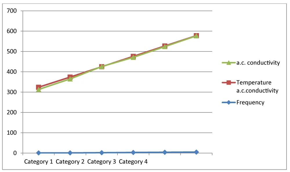
Figure 4: A graph between frequency, temperature and a.c. conductivity.
The theoretical and virtual calculations through equation (4) and (5) provide extensive results for the normal conductivity and a.c. conductivity of the material. At low temperature, there is no significant change in conductivity. The curve shows an exponential decrease, as in the original formula for dielectrics, while the modified formula signals the decrease in conductivity. The graphical variation in Fig.1 represents the decrease in normal conductivity in the vicinity of a short interval of temperature, whereas the theoretical formula represents the exponential change with temperature. In Figure 2, a.c. conductivity goes on increasing starting from high temperature above 1000oC and follows the linearity. The experimental graphs shown in Figure. 3(a) and Figure. 3(b) show the frequency versus ac conductivity and temperature vs a.c conductivity, respectively. As we know, a.c. conductivity is a function of frequency; as frequency increases, a.c. conductivity increases. The experimental graphs shown in Figure 3(a,b) show that a.c. conductivity increases as the temperature increases. For the variable 1.4 kelvin, its value appears as 714.28, for which the corresponding a.c. conductivity 0.1 per ohm per cm. Similarly, for the variable 1.8, the temperature is 625, corresponding to the a.c. conductivity is 0.01 per ohm per cm. Even our theoretical model, as shown in Figure 4, shows that as the temperature is 323 K, the a.c. Conductivity is -11 order, and when it is 373K, a.c. conductivity is -9. It shows the theory and experiment are logically consistent in the same direction. It is due to thermally activated charge carriers. The a.c. conductivity of ferroelectric material increases with increasing frequency. It can be seen through Arrhenius behavior: The proposed model of a.c. conductivity is explained by Jonscher’s universal power law, i.e.,
Where A = temperature –dependent constant, n=frequency exponent.
This equation also explains that the normal conductivity increases at low frequency and a.c. conductivity increases at high frequency because of the hopping of charge carriers.
The rigorous and virtual calculation of a.c. conductivity of lead-free ceramics ABO3-type ferromaterials exhibits good conducting nature, as to why ionic polarization increases. It helps predict less energy consumption as well as reducing the pollution rate. Since ABO3 materials have high a.c. conductivity, it can be used in sensors, ultrasonic transducers, and microphones. It can also be used in highly efficient photovoltaic cells.
Future aspects of research
1. To study the mixed dielectric properties and specific heat capacity of the multilayer ceramic materials.
2. How to save energy consumption of energy.
3. Optoelectronic properties in polarization.
4. Temperature sensing.
I am indebted to the Society of Materials Chemistry and R.N.P. Choudhary’s research work on ceramic materials. The proper and continuous guidance with valuable lectures on ceramic materials by the former head and Professor of the University Department of Physics influenced me to work in the existing field.
Conflict of interest statement
A new ceramic constant σc leads to yield the remarkable varying a.c. conductivity controlling the density.
Author’s contribution
The author’s contributions are Calculation of a.c. conductivity controlling the frequency and temperature, and the conceptual ideas of ceramic and lead-free ceramic materials.
Data availability
The a.c. conductivity σac is taken from equation 2 and normal conductivity from equation 4 with varying temperature.
- Ye ZG. Handbook of dielectric, piezoelectric and ferroelectric materials: synthesis, properties and applications. Boca Raton (FL): CRC Press; 2008. Available from: file:///C:/Users/ADMIN/Downloads/Z._Ye_Handbook_of_Advanced_Dielectric_PiezoelecBookFi.org.pdf
- Astin IG, Mott NF. Polarons in crystalline and non-crystalline materials. Adv Phys. 1969;18:41-102. Available from: https://doi.org/10.1080/00018736900101267
- Sharma GD, Roy M, Roy MS. [Article title not provided]. Mater Sci Eng B. 2003;104:15.