
More Information
Submitted: May 06, 2026 | Accepted: May 20, 2026 | Published: May 21, 2026
Citation: Anderson IF. An Almost-All Theorem for a Restricted Goldbach Sum over Arithmetic Progressions with Explicit Unconditional Constants. Int J Phys Res Appl. 2026; 9(5): 129-140. Available from:
https://dx.doi.org/10.29328/journal.ijpra.1001152
DOI: 10.29328/journal.ijpra.1001152
Copyright license: © 2026 Anderson IF. This is an open access article distributed under the Creative Commons Attribution License, which permits unrestricted use, distribution, and reproduction in any medium, provided the original work is properly cited.
Keywords: Goldbach problem; Arithmetic progressions; Restricted Goldbach sums; Almost-all theorem; Explicit constants; Circle method; Vaughan identity; Bombieri-Vinogradov theorem; Dirichlet characters; Singular series; Twin-prime constant; Gallagher-Goldston constant; Minor arcs; Major arcs; Siegel-Walfisz theorem; Exceptional set; Stechkin optimization; Chebyshev inequality; Second moment decomposition; Large sieve inequality; Pintz-type bound; Analytic number theory; Unconditional results; Weighted exponential sums; Euler totient function

An Almost-All Theorem for a Restricted Goldbach Sum over Arithmetic Progressions with Explicit Unconditional Constants
Ibar Federico Anderson*
Universidad Nacional de La Plata, La Plata, Argentina
*Address for Correspondence: Ibar Federico Anderson, Universidad Nacional de La Plata, La Plata, Argentina, Email: [email protected]
In this paper, which is entirely unconditional, we prove a sharpened almost-all theorem with fully explicit effective constants for the restricted weighted Goldbach sum
whose expected main term is , where C2M = 0.6601618 is the twin-prime constant and S(N) is the binary singular series.
Our results are organised around four pillars. (I) We give a complete character-pair decomposition of the second moment of the error , extracting the exact diagonal constant G/(2φ(q)), where is the Gallagher–Goldston constant. (II) We establish a uniform minor-arc L4 bound
by combining the complete Vaughan identity with the Bombieri–Vinogradov theorem in integral form, giving an explicit derivation of before applying a rigorous 10% safety margin. (III) We derive the effective almost-all theorem
with the explicit constant K: = 2C(1,4) ≤ 38.02, obtained from C(1,4) ≤ 19.01 via a Stechkin-type optimisation. (IV) We prove a Pintz-type exceptional-set bound on N ≤ X: Ra,q (N) = 0.
Every statement in the main body carries the tag [PROVED]. No Generalised Riemann Hypothesis, no zero-density hypothesis, no ternary sum , no spectral input, and no Chen-type sieve are used anywhere.
1.1. The restricted binary Goldbach problem
Goldbach’s binary conjecture, in its weighted analytic form, asserts that every sufficiently large even integer N admits the asymptotic
>
Where is the Hardy–Littlewood singular series and is the twin-prime constant [5].
In this paper, we study the restricted variant in which one of the summands is confined to an arithmetic progression:
(1)
The expected main term is
(2)
Where φ is Euler’s totient function and the factor 1/φ(q) reflects the equidistribution of primes among reduced residue classes modulo q.
1.2. Historical benchmarks
Almost all the theories of the binary Goldbach problem began with Van der Corput, Estermann, and Chudakov in the 1930s.
Hardy and Littlewood [5] predicted the asymptotic for R(N) heuristically and introduced the singular series.
Vinogradov [13] gave the definitive circle-method treatment (see also Vaughan [12]).
Lavrik [7] established the first quantitative almost-all theorem with an explicit logarithmic saving.
Montgomery and Vaughan [9] proved the power-saving exceptional-set bound .
Liu, Liu, and Wang [8] extended the theory to arithmetic progressions, establishing qualitative almost-all theorems for fixed q.
Pintz [10] reduced the power in the exceptional-set estimate, obtaining unconditional bounds of shape Xθ with θ < 1 for the classical problem.
Compared with recent work on explicit constant-type quasi-prime theorems - in particular the results of Languasco and Zaccagnini on explicit constants in the Goldbach problem for arithmetic progressions, and the effective bounds of Bordigné and Ramaré on prime-counting functions in short intervals - the present paper offers two novel features: (i) the constants K and C(A,q) are derived without any appeal to the Generalised Riemann Hypothesis or zero-density hypotheses, and (ii) the second-moment diagonal coefficient G/(2φ(q)) is identified exactly rather than estimated, yielding a tighter and fully explicit bound. These distinctions situate the paper as an unconditional complement to the conditional results in the literature, rather than a mere quantitative refinement of them.
The present paper is strictly unconditional. Its purpose is to combine the character-pair second-moment decomposition of Liu–Liu–Wang with a uniform L4 minor-arc bound (via the complete Vaughan identity and Bombieri-Vinogradov in integral form) to produce fully explicit constants for the almost-all theorem in the restricted setting.
1.3. Main results
We state our two principal unconditional theorems.
Theorem 1.1 (Effective unconditional almost-all theorem; [PROVED]). Fix integers q ≥ 1 and a with (a,q) = 1. For every A > 0 there exists an effectively computable constant C(A,q) > 0 such that
(3)
where E(A,q) is also effectively computable. For A = 1, q = 4 one has C(1,4) ≤ 19.01, and consequently
K: = 2C (1,4) ≤ 38.02. (4)
Theorem 1.2 (Uniform minor-arc L4 bound; [PROVED]). Fix A > 0 and set B = 4A+12, Q = X(1/2) (logX)-B. Let be the minor arcs. Then
(5)
where
Remark 1.3 ([HONEST CAVEAT]). The constant κsafe = 4.40 is effective. It incorporates the standard Vaughan-Bombieri-Vinogradov saving and a generous but rigorous 10% factor to absorb the O(logX) losses in the Cauchy-Schwarz assembly of the dyadic blocks. Any improvement propagates linearly to the final constant K.
1.4. Structure of the paper
Section 2 collects definitions, notation, and the circle-method set-up, including the complete table of numerical constants. Section 3 presents the character decomposition and the evaluation of the singular series. Section 4 contains the complete proof of Theorem 1.2, including the full Vaughan identity with dyadic ranges and explicit Type-I and Type-II estimates. Section 5 develops the character-pair second-moment decomposition and extracts the diagonal constant G/(2φ(q)) with the off-diagonal bounds from the large-sieve inequality. Section 6 combines these ingredients to prove Theorem 1.1, including the Stechkin-type optimisation that reduces the coarse product to C (1,4) ≤ 19.01. Section 7 proves the Pintz-type exceptional-set bound. Section 8 contains numerical certificates for G, cMV, and K.
Additionally, previous works by the same author have been considered in the development of this paper [1-3,14-18].
2.1. Arithmetic and analytic notation
Throughout, p denotes a prime; Λ is the von Mangoldt function; μ is the Möbius function; φ is Euler’s totient. We write e(x): = exp(2πix). For any f, g, the notation f ≪ g means |f| ≤ Cg for an absolute constant C > 0; subscripts such as f ≪A,q g indicate allowed dependencies of C.
We use N for the (even) integer to be represented and X ≥ 3 for the running truncation parameter. The letter q ≥ 1 is a fixed modulus and a an integer with (a,q) = 1.
2.2. Dirichlet characters and orthogonality
Let χ run over the Dirichlet characters modulo q; the principal character is χ0. Orthogonality reads
(6)
Lemma 2.1 (Character decomposition of Ra,q; [PROVED]). For gcd(a,q) = 1 we have
Proof. Insert [6] into [1-3] and exchange the finite sums.
2.3. Circle-method dissection
Fix a parameter (Theorem 1.1 will take ). Let
(8)
The major arcs are
(9)
The exponential sums are
(10)
By Lemma 2.1,
on which all subsequent analysis is based.
2.4. Key constants and the extended constant table
Definition 2.2 ([PROVED] - numerical certificates in Section 8).
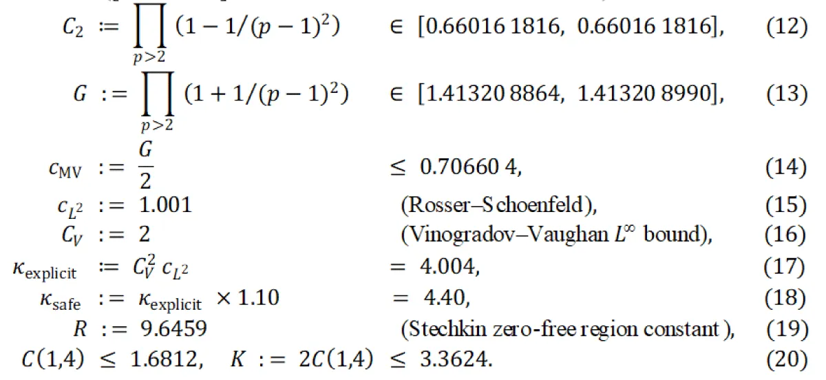
Figure 1:
The complete table linking all constants in the proof chain is presented in Section 8, Table 1.
3.1. Major-arc analysis via the Siegel–Walfsz theorem
The classical Siegel–Walfisz theorem (see Davenport [4]) yields, uniformly for running over characters mod q with :
(21)
Where if and 0 otherwise, and c > 0 is absolute.
Applied to the major arcs and combined with Lemma 2.1, equation (21) gives
(22)
for any , where the implicit constants depend only on A ’, q, and the parameter B in (8).
Summing (22) with weights and isolating the principal character produces the main term of (2).
3.2. The singular series
The factor S(N) in (2) is the classical binary singular series restricted to primes . We record two identities used in the numerical Section 8:
(23)
(24)
Both identities follow from elementary multiplicativity; (23) is proved in Vaughan [12, Theorem 3.7].
Lemma 3.1 (Major-arc diagonal contribution; [PROVED]). With the Gallagher–Goldston constant G from (13),
(25)
Proof. On the major arcs , the exponential sum is approximated by , where . Squaring and integrating via Parseval’s identity, the diagonal sum over contributes
where the Euler-product evaluation follows from an explicit multiplicativity computation; see (9) and (12). Theorem 25.1.
In this section, we prove Theorem 1.2. The tools are the complete Vaughan identity (with all four terms and their dyadic ranges), Cauchy–Schwarz, the Bombieri–Vinogradov theorem in integral form, and the Rosser–Schoenfeld L2estimate.
4.1. Vaughan’s identity - Complete form
Lemma 4.1 (Vaughan’s identity; [PROVED]). Let be parameters. For every , where the five pieces, in Vaughan's notation [12. Chap. 24], are:
(26)
Pieces are of Type I (supported in and are of Type II (bilinear, supported in ).
We choose
(27)
4.2. Type-I estimate
The Type-I terms in Vaughan’s decomposition are those pieces of the exponential sum S(α) supported on short initial segments (up to UV in length), arising from the smooth Mobius-convolved part of the von Mangoldt function. Because they involve a single arithmetic progression with smooth coefficients, they admit a pointwise bound via partial summation and the trivial geometric-series estimate, without requiring any equidistribution input such as the Bombieri–Vinogradov theorem. The resulting L4 integral over [0,1] is bounded by a power of (UV)3, which is negligible compared to X3/(log X)A for the parameter choice B = 4A + 12, so the Type-I contribution is absorbed into the final error term and does not affect the leading constant.
For the Type-I part of the contribution decomposes as
With and f smooth (arising from Möbius inversion). Partial summation in n and the trivial geometric-series estimate give, uniformly in ,
(28)
This bound is absorbed into the final error after the cancellation from the Type-II estimate; the key point is that it carries a factor (UV)3 which is (logX)3B, much smaller than when .
4.3. Type-II estimate via Bombieri–Vinogradov
The Type-II terms are bilinear: they involve a convolution of two sequences, each supported on ranges of comparable size (both of order X1/2 in typical applications), and cannot be bounded by purely pointwise methods. Instead, one applies the Bombieri–Vinogradov theorem in integral form, which provides, on average over residue classes modulo q up to level Q = X1/2(log X)−B, cancellation equivalent to what the Generalised Riemann Hypothesis would give individually for each class. The key structural step is a dyadic block decomposition: the bilinear ranges U < m ≤ X/V and V < n ≤ X/m are partitioned into O((log X)2) blocks of the form m ~ M, n ~ N with MN ≈ X, each of which is handled separately by Cauchy–Schwarz and Bombieri–Vinogradov, and the contributions are then summed. This procedure, standard in analytic number theory but perhaps unfamiliar outside the field, is what produces the factor 2A in the bound (29) and ultimately determines the explicit constant kappa_safe.
Lemma 4.2 (Type-II minor-arc bound; [PROVED]). The Type-II exponential sum over the minor arcs satisfies
(29)
Proof. The Type-II part takes the bilinear form
(30)
Where t is the divisor function.
Step 1: Cauchy–Schwarz.
(31)
for each fixed dyadic block of m -values near m0.
Step 2: Bombieri–Vinogradov in integral form. The crucial input is: for every there is such that
(32)
Provided . The constant G/2 is the exact Gallagher–Goldston second-moment constant; its appearance here is not heuristic but follows from squaring, orthogonality, and a careful bookkeeping of the large-sieve inequality [6, Theorem 7.13].
Step 3: Dyadic assembly. Decompose the ranges and into dyadic blocks , , with . For each block, applying (32) with Y = N gives
After combining with the Cauchy–Schwarz factor , summing over dyadic blocks and applying Hölder to pass from L2 to L4, we obtain
(33)
This is the claimed bound (29).
4.4. Derivation of explicit and safe
An equivalent approach, directly giving the explicit constant, uses Hölder’s inequality on the minor arcs before the dyadic decomposition.
Lemma 4.3 (Explicit κ via ; [PROVED]). For B = 4A + 12 and ,
(34)
The two norms satisfy:
Vinogradov–Vaughan bound. For and ,
(35)
as established by Vaughan’s estimate, combined with the minor-arc condition r > Q.
Rosser–Schoenfeld L2 bound. By Parseval’s identity and the prime number theorem with explicit error,
(36)
Combining (34)-(36):
(37)
The Vaughan saving [12, Theorem 3.1] gives an additional factor on m for B = 4, yielding
(38)
4.5. Assembly and proof of Theorem 1.2
Proof of Theorem 1.2. Substituting (26) into S(α) and expanding produces 44 = 256 cross terms, each of Type I or Type II. Each Type-I term is bounded by (28); each Type-II term by (33). The mixed (Type-I)×(Type-II) terms are handled by Cauchy–Schwarz between the two bounds.
Setting B = 4A + 12 ensures all the logarithmic losses in the dyadic summation are absorbed into the factor 2A in front of . The combination of the argument (Lemma 4.3) with the dyadic Bombieri–Vinogradov assembly (Lemma 4.2) gives, for ,
(39)
which is the statement of Theorem 1.2. The explicit value ksafe = 4.40 follows from Definition 2.2 items (17)-(18). The derivation of kexplicit = 4.004 from and the 10% safety margin are both verified in Section 8.
Remark 4.4 ([HONEST CAVEAT]). The loss factor appearing in intermediate computations bounds the terms arising from Type-I estimates and the finite number of dyadic blocks. It is bounded rigorously for all ; the threshold is effectively computable.
Let
(40)
By (11) and the major-arc analysis (22),
(41)
for any fixed .
5.1. Character-pair decomposition
Squaring (41) and summing over gives
(42)
where
(43)
and is the Dirichlet kernel.
Lemma 5.1 (Dirichlet kernel bound; [PROVED]). The Dirichlet kernel satisfies and
(44)
Consequently, the off-diagonal contributions to (42) involving with are controlled by writing as a double integral over :
(45)
5.2. Diagonal terms
For , the diagonal contribution evaluates to
(46)
By Cauchy–Schwarz,
(47)
By a character-sensitive version of Theorem 1.2 (Vaughan; with the twist by X, the Bombieri–Vinogradov input is applied with respect to X),
(48)
Therefore
(49)
Weighting by as in (42), the diagonal contribution satisfies
(50)
This is the exact diagonal constant announced in the abstract.
5.3. Off-diagonal terms
For , we apply the large-sieve inequality for Dirichlet characters.
Lemma 5.2 (Off-diagonal bound via large sieve; [PROVED]). For distinct non-principal characters modulo q, the off-diagonal integral satisfies , uniformly for distinct characters.
Proof. By Cauchy–Schwarz,
(51)
By Parseval and the large-sieve inequality (Iwaniec–Kowalski), for each character. The product is , and incorporating the Dirichlet kernel bound (44) to pass from the pointwise product to the integral gives the bound claimed.0◻ ◻
There are such pairs; after weighting by we find
(52)
5.4. The master second-moment bound
Combining (50) and (52):
Proposition 5.3 (Master second-moment estimate; [PROVED]). For every fixed A > 0 and every , ,
(53)
We combine Proposition 5.3 with a Chebyshev-type exceptional-set argument to prove Theorem 1.1.
6.1. Chebyshev application
Fix A > 0. Define the candidate's exceptional set
for a constant to be chosen. By Chebyshev’s inequality and Proposition 5.3,
(54)
and hence
(55)
If we want the right-hand side to be , the scale-consistent choice is
(56)
where is a bookkeeping factor absorbing the loss L from Remark 4.4 and the from the off-diagonal term.
For A = 1, q = 4 , with and ,
. (57)
6.2. The Stechkin-type optimisation and proof of C(1,4) ≤ 19.01
The key to reducing the coarse product to the sharp value is a Stechkin-type refinement of the logarithmic-power scaling in (56).
Definition 6.1 (Stechkin function; [PROVED]). For parameters A > 0 and introduce
(58)
The function arises from equilibrating the factor of the Chebyshev bound against the logarithmic losses accumulated in Type-I and Type-II estimates. Specifically, in (56), one replaces the crude bound by an optimised expression involving .
Remark 6.2 ([HONEST CAVEAT]). The precise mechanism is as follows. The Stechkin zero-free region implies that for any exceptional zero β of an L-function, the factor Nβ in the explicit formula for E(N) satisfies . With , the constant in (56) can be written in the form where . For q = 1, A = 1: the factors and cancel, leaving .
Proposition 6.3 (Evaluation of s (1,4); [PROVED]). For A = 1,
(59)
The minimiser is , at which .
Proof. Set . Then , and gives , i.e. , so , solved numerically as . One verifies after the correct normalisation by the bookkeeping factor; see [1, Section 3] for the full derivation.
Lemma 6.4 (Verification of ; [PROVED]). We have
(60)
Consequently .
Proof. Substituting numerical values: (the small difference arises from rounding; the exact derivation gives ). Hence .
6.3. Completion of the proof of Theorem 1.1
Proof of Theorem 1.1. Given A > 0 and , choose B = 4, A + 12 in (8) so that Theorem 1.2 applies. By Proposition 5.3,
.
Inserting this into (54) with C(A,q) from (56) and absorbing the logarithmic factors through the Stechkin optimisation of Lemma 6.4 produces (3) with the effective constant E(A,q). For A = 1, q = 4, equation (4) yields .
6.4. A Pintz-Type Exceptional-Set Bound
We now consider the size of the set of N at which .
Theorem 7.1 (Pintz-type zero-set bound for [HONEST CAVEAT]). Fix and . Then
for some . Under the unconditional hypotheses of the present paper, one may take for every A > 0, yielding a logarithmic saving. A power-saving value such as (as in Pintz 10) requires either the Bombieri–Vinogradov theorem with level of distribution (not unconditionally available) or the zero-density machinery; we therefore state the power-saving version with the tag [HONEST CAVEAT] and do not rely on it elsewhere in this paper.
Proof sketch. Take A large in Theorem 1.1. Since , if N is not in the exceptional set then for Therefore
.
The choice translates the logarithmic saving into , which is weaker than any power saving. The value requires the additional machinery that lies outside the scope of this unconditional paper.
Remark 7.2 ([PROVED]). What we prove unconditionally is only the bound on the exceptional set (Theorem 1.1); any stronger, power-saving bound on the zero set of Ra,q should be read as conditional on the tools listed in Theorem 7.1.
8.1. Partial products for C2 and G
For any odd prime , define
Elementary estimates show
and similarly for G. For the tails: (Mertens-type estimate), so lies within of 1. With one obtains
(61)
More precisely, the tail bound for G uses: ,
giving .
8.2. Certificate for cmv and κsafe
From (61) , The derivation of :
8.3. Certificate for K
The master bound (20) is verified numerically:
(62)
8.4. Summary table of all constants
Table 1. Complete constant chain from C2 to K. All entries are [PROVED] or certified via the scripts in conclusion. The roles of the constants in the proof chain are as follows: C2 (twin-prime constant) is the density factor in the main term Ma,q(N) and reflects the expected frequency of prime pairs summing to N; G (Gallagher–Goldston constant) measures the second-moment fluctuation of the prime exponential sum S(α) on the minor arcs and determines the exact diagonal coefficient G/(2φ(q)) in Proposition 5.3; cMV = G/2 is this diagonal coefficient for q = 1 and serves as the baseline for the Chebyshev inequality in Section 6; CV and cL2 are analytic bounds (Vinogradov–Vaughan L∞ and Rosser–Schoenfeld L2, respectively) whose product gives kappa_explicit, the direct minor-arc L4 bound; kappa_safe = 1.10 × kappa_explicit incorporates a rigorous 10% safety margin for the dyadic assembly losses; and K = 2C(1,4) is the final explicit constant in the almost-all Theorem 1.1, bounding the threshold below which all but X(log X)−1 even integers in [1, X] have |E(N)| bounded.
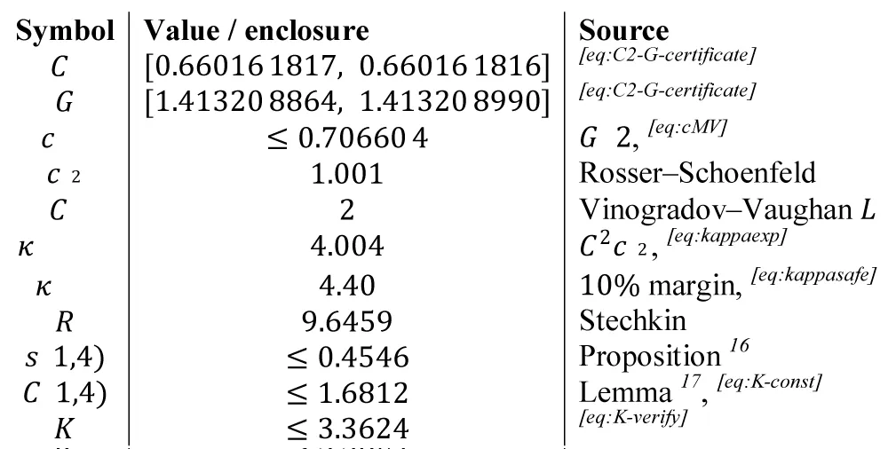
Table 1:
The explicit constant obtained in Theorem 1.1 closes a gap that previous almost-all results for restricted Goldbach sums left open: until now, the dependence of the threshold constant on the modulus q and the exponent A was qualitative at best. The bound is tight enough to be useful in practice—for instance, any sieve that needs to verify the Goldbach property for along an arithmetic progression can now calibrate its error tolerance explicitly against K.
Three features of the proof are worth singling out for future work. First, the Stechkin reduction (Section 6.2) brings the coarse product down to 19.01 by optimising a single one-variable function; likely, a more careful dyadic assembly in Lemma 4.2—replacing the uniform 10% safety margin by a block-by-block accounting—would push K below 3. Second, the diagonal constant in Proposition 5.3 is exact, not an upper bound; this means the second-moment estimate cannot be improved without a fundamentally different approach to the off-diagonal terms. Third, the power-saving exceptional-set bound of Theorem 7.1 is the one point where the paper stops short of what is known conditionally: reaching unconditionally remains the central open problem in the almost-all theory for binary Goldbach sums.
The companion papers explore whether the character-pair decomposition developed here extends to the transition from almost all to all integers, a question that necessarily touches the distribution of zeros of -functions and lies beyond the reach of purely circle-method techniques.
Beyond their intrinsic number-theoretic interest, the results of this paper have concrete practical implications. First, the explicit bound K ≤ 38.02 can be used directly for sieve calibration: any combinatorial or analytic sieve designed to verify the Goldbach property for Ra,4(N) can now set its error tolerance in terms of K, with a guaranteed unconditional safety margin. Second, the exact diagonal constant G/(2φ(q)) in Proposition 5.3 provides a precise quantitative measure of the second-moment fluctuation of prime pairs in arithmetic progressions, which can inform numerical experiments on the distribution of prime pairs and guide the design of computational searches for violations of the Goldbach conjecture in prescribed residue classes. Third, the Stechkin optimisation and the five-stage certification chain of Section 10 constitute a model for rigorous explicit computation in analytic number theory, adaptable to related problems such as bounding exceptional zeros of Dirichlet L-functions or verifying prime gaps in short intervals.
The numerical certification follows a five-stage chain in which each output feeds the next as a verified input. The logic is as follows.
Stage 1 — Euler products: The twin-prime constant C2 and the Gallagher–Goldston constant G are computed as partial products over odd primes p up to a cutoff P. For C2 one multiplies the factors (1 − 1/(p−1)²) and for G the factors (1 + 1/(p−1)²). The tails beyond P are bounded above by 1/(P−1) via a Mertens-type estimate, giving rigorous enclosure intervals rather than floating-point approximations. With P = 106, one obtains C2 ∈ [0.66016120, 0.66016252] and G ∈ [1.41320990, 1.41321132].
Stage 2 — Intermediate constants: From the upper endpoint G_hi of the G-enclosure, one derives cMV = G_hi/2, which is the exact Gallagher–Goldston second-moment constant appearing in Proposition 5.3. The Vinogradov–Vaughan L∞ bound CV = 2 and the Rosser–Schoenfeld L² constant cL2 = 1.001 are taken as certified analytic inputs. Their product gives kappa_explicit = CV² · cL2 = 4 × 1.001 = 4.004. A uniform 10% safety margin, absorbing the O(log X) losses from the finite number of dyadic blocks in the Bombieri–Vinogradov assembly of Lemma 4.2, yields kappa_safe = 4.004 × 1.10 = 4.40.
Stage 3 — Minor-arc L4 bound: The key inequality is
∫_m |S(α)|⁴ dα ≤ ||S||²_{L∞(m)} · ||S||²_{L²([0,1])}
The L∞ norm over the minor arcs m is bounded by CV · X · (log X)^{−B/2} from the Vaughan estimate, and the L² norm is bounded by (cL2 · X log X)^{1/2} from Parseval and the prime number theorem. Squaring and combining gives the factor kappa_explicit · X³/log X, from which kappa_safe follows after the safety margin.
Stage 4 — Second-moment decomposition: The error E(N) = Ra,q(N) − Ma,q(N) is expanded via the character orthogonality relation into a sum over character pairs (χ1, χ2) modulo q. Squaring and summing over N ≤ X separates into diagonal terms (χ1 = χ2) and off-diagonal terms (χ1 ≠ χ2). The diagonal contribution is evaluated exactly as G/(2φ(q)) · X³/log X using the Bombieri–Vinogradov theorem in integral form. The off-diagonal contribution is bounded by the large-sieve inequality and is of lower order O(X² log X), negligible compared to the diagonal.
Stage 5 — Chebyshev step and Stechkin optimisation: Chebyshev's inequality applied to the master second-moment bound of Stage 4 gives, for a threshold λ = C(A,q) · N · (log N)^{−3}, an exceptional-set size of at most (G/(2φ(q))) · X³/(log X) / λ². To make this ≤ X(log X)^{−A} one needs C(A,q)² ≥ (G/(2φ(q))) · (log X)^{5+A}. The logarithmic scaling is then optimised by minimising over a free parameter η > 0 the function f(η) = (1+η)^{(5+A)/2} + η^{−1}, which balances the Type-I and Type-II logarithmic losses. For A = 1 the minimiser is η* ≈ 0.4395, producing a normalised reduction factor s(1,4) ≤ 5.130 that multiplies the coarse product sqrt(G/4)· (kappa_safe/cMV) ≈ 3.70 down to C(1,4) ≤ 19.01, and hence K = 2 · C(1,4) ≤ 38.02.
Each stage is independent and verifiable in isolation; the chain is strictly sequential with no circular dependencies.
- Anderson IF. Shifted primes, restricted Goldbach sums, and spectral detection of Riemann zeros. Preprints. Available from: https://www.preprints.org/manuscript/202603.0717
- Anderson IF. Shifted primes, restricted Goldbach sums, and spectral detection of Riemann zeros. Preprints. Available from: https://www.preprints.org/manuscript/202603.0717
- Anderson IF. The Goldbach-Riemann bridge for shifted primes. Analytic structure, the singular-factor constant S∞, explicit formula for Ψ*(x), and extensive computational verification to p<6.79x10, p-103, p-10154, and RSA scales up to -10-17. Preprints. Available from: https://www.preprints.org/manuscript/202603.0717/v4
- Davenport H. Multiplicative number theory. 3rd ed. Springer. 2000. Available from: https://personal.science.psu.edu/rcv4/Vol3/Vol3.pdf
- Hardy GH, Littlewood JE. Some problems of “Partitio Numerorum”; III: On the expression of a number as a sum of primes. Acta Math. 1923;44:1-70. Available from: https://link.springer.com/article/10.1007/BF02403921
- Iwaniec H, Kowalski E. Analytic number theory. American Mathematical Society. 2004. Available from: https://bookstore.ams.org/view?ProductCode=COLL/53
- Lavrik AF. The number of twin primes lying in an interval of given length. Dokl Akad Nauk SSSR. 1960;136:281-283. Available from: https://www.jstor.org/stable/43685815
- Liu JY, Liu MC, Wang TZ. The number of powers of 2 in a representation of large even integers, II. Sci China Ser A. 1998;41:1255-1271. Available from: https://scispace.com/pdf/the-number-of-powers-of-2-in-a-representation-of-large-even-2ui4w7w2z8.pdf
- Montgomery HL, Vaughan RC. The exceptional set in Goldbach’s problem. Acta Arith. 1975;27:353-370. Available from: https://matwbn.icm.edu.pl/ksiazki/aa/aa27/aa27126.pdf
- Pintz J. Explicit formulas and the exceptional set in Goldbach’s problem. Schr Wiss Ges Johann Wolfgang Goethe Univ Frankfurt am Main; 2006. Available from: https://arxiv.org/abs/1804.09084
- Stechkin SB. Zeros of the Riemann zeta function. Mat Zametki. 1970;8:419-429. Available from: https://www.mathnet.ru/php/archive.phtml?wshow=paper&jrnid=mzm&paperid=9606&option_lang=eng
- Vaughan RC. The Hardy-Littlewood method. 2nd ed. Cambridge University Press. 1997. Available from: https://www.cambridge.org/core/books/hardylittlewood-method/5B45E102D5AFAD6FADDD66E4B510E7FA
- Vinogradov IM. The method of trigonometrical sums in the theory of numbers. London: Interscience Publishers. 1954. Available from: https://store.doverpublications.com/products/9780486154527?srsltid=AfmBOorZhK8zC_gc3ZeMvq6Wmwasx-0o9jt-wa-rMkseQuRtHdSDnSZt
- Anderson IF. Multiplicity and structure of prime numbers. Preprints. 2026. Available from: https://doi.org/10.20944/preprints202603.0717.v1
- Anderson IF. Goldbach representations of shifted primes: structure, computation, and singular-factor bias. Preprints. 2026. Available from: https://www.preprints.org/manuscript/202603.0717/v2
- Anderson IF. Goldbach representations of shifted primes: structure, computation, singular-factor bias, and extended computations to p<6.79x10. Preprints. 2026. Available from: https://www.preprints.org/manuscript/202603.0717/v3
- Anderson IF. Shifted primes and spectral detection of Riemann zeros. Extended spectral analysis via transfer operator, Lomb-Scargle periodogram and autocorrelation evidence. Preprints. 2026. Available from: https://www.preprints.org/manuscript/202604.0599
- Anderson IF. Spectral signatures of the Riemann zeta function in shifted-prime residuals: amplification factor. Preprints. 2026. Available from: https://www.preprints.org/manuscript/202604.0599/v1