Review Article
Finite-time thermodynamics: Realizability domains of thermodynamic systems and P. Salamon’s problem of efficiency corresponding to maximum power output of the system
Tsirlin AM and Sukin IA
Ailamazyan Program Systems, Insitute of Russian Academy of Sciences, Pereslavl-Zalessky, Russia
*Address for Correspondence: Tsirlin AM, Ailamazyan Program Systems, Insitute of Russian Academy of Sciences, Pereslavl-Zalessky, Russia, Email: [email protected]
Dates: Submitted: 03 September 2018; Approved: 15 October 2018; Published: 15 October 2018
How to cite this article: Tsirlin AM, Sukin IA. Finite-time thermodynamics: Realizability domains of thermodynamic systems and P. Salamon’s problem of efficiency corresponding to maximum power output of the system. Int J Phys Res Appl. 2018; 1: 052-066. DOI: 10.29328/journal.ijpra.1001004
Copyright: © 2018 Tsirlin AM, et al. This is an open access article distributed under the Creative Commons Attribution License, which permits unrestricted use, distribution, and reproduction in any medium, provided the original work is properly cited.
Keywords: Fusion reactors; Dense plasma focus; Nanosecond neutron pulses; Neutron activation diagnostics; Time-of flight spectral diagnostics

Abstract
The paper analyses performance boundaries of systems converting the heat energy into the mechanical or separation work. Authors approach this problem from the view-point of the finite-time thermodynamics. Using thermodynamic balance equations, authors provide the algorithm for calculation of realizability domain for such systems. The paper shows that the performance of these systems is the upper bounded function of the heat flux, assuming that heat and mass transfer coefficients are given. Authors present sufficient conditions under which the efficiency (specific heat flux per unit of the useful flux) of the system does not depend on kinetic coefficients when operating in the maximum performance mode. The paper shows how to use these conditions to optimally choose the separation order for multicomponent distillation.
Introduction
Systems converting the heat energy into some kind of work are very common in the industry. It is not only heat engines but also systems separating liquid and gas mixtures. For the latter case a system produces a separation work, increasing the Gibbs energy of outgoing flows compared to ingoing ones. The expression for the efficiency of a system follows from thermodynamic balance equations: energy balance, material balance and entropy balance. The geometry of the realizability domain can also be determined using these equations. The entropy balance equation contain σ which is equal to the overall energy dissipation within a system. Its value is always non-negative.
The realizability domain on the plane where the x-axis corresponds to heat flux and the y-axis corresponds to the performance value is getting narrower when σ increases. The upper bound of this domain would be obtained if one assumed σ = 0. The bounding curve in this case is a straight line has the slope equal to the efficiency of the reversible process ηrev. It is the Carnot efficiency for the heat engine with the sources having constant temperature [1]. This efficiency is equal to the ratio of the Carnot efficiency and the specific separation work for the distillation column having temperatures within the reboiler and the reflux drum constant, when the performance is assumed to be the feed flux [2,3]. Temperatures within the reboiler and the reflux drum play the role of sources’ temperatures.
If one estimated the energy dissipation from below, obtaining its relation to the fluxes, kinetic coefficients etc., the realizability domain would become narrower and its geometry would change. Its qualitative characteristics depends on the nature of the target flow and energy flow. It will be shown below that if the energy flow is the the heat energy one and the target flow is the electrical or mechanical energy one, the realizability domain will be very close to the concave bounded parabola, but if the energy flow is the mechanical work one and the target flow is the heat energy one, the realizability domain is concave but unbounded.
The first works researching performance boundaries of the irreversible thermodynamics systems were the papers, considering cycles of heat engines of the nonzero power output ([4,5] and many others). This area still remains of great interest and there are many modern writings on the subject [6-18]. The papers such as [7-10,12,16,17] consider special cases of kinetic laws, the others (for example, [11,14,18]) solve the problem for the general formulation of kinetics. The general proof of the independence of the system efficiency of kinetic coefficients has hitherto been unknown. The given paper tries to address this issue.
The limited values of heat transfer coefficients αi between sources and the working body were the irreversible factor influencing the power output of the engine. Due to this the power output of the engine p were increasing with the increase of the heat flux and the corresponding irreversibility at first, then reaching its maximum p∗ and then decreasing to zero.
For the linear kinetics of heat transfer
(1)
where Tf and Tr are temperatures of a source and the working body respectively, the power output p of the heat engine relates to the heat flux from the hot source q+ as [19]
. (2)
Here and α− are coefficients of heat transfer between sources and the working body.
The expression within brackets in (2) is the efficiency value for the given power output. This output is bounded and could not be greater than
, (3)
The efficiency value will approach the Carnot efficiency ηrev if the power output strives for zero for the mode of maximum power output it is equal to the value obtained first by Novikov and later by Curzon and Ahlborn
.
The value ηnca does not depend on heat transfer coefficients unlike the maximum power output. It depends only on the efficiency of the reversible process
ηnca = (4)
The maximum difference between ηrev and ηnka is reached when the ratio of absolute temperatures of sources T−, T+ is equal to 0.25. In this case ηrev = 0.75 and ηnca = 0.5.
If the heat transfer laws is such that the heat flux is proportional to the difference of inverse values of temperatures 1/T− − 1/T+ (thermodynamic driving force), the efficiency value corresponding the maximum power output does not depend on α+,α− too. Its value is equal to the half of the Carnot efficiency.
Systems consuming the heat energy will be called the thermal ones. They convert the heat energy into the separation work. The most common thermal system is the distillation column. The efficiency value is equal to the ratio of the feed flux to the heat one for the distillation of ideal binary mixtures ([20,21]). In the reversible process (the power output is arbitrarily low).
, (5)
where AG is the specific separation work which is equal to the difference of the Gibbs energy of outgoing flows and the feed one; TD, TB are temperatures in the reflux drum and the reboiler.
The power output of the column increases with the increase of the heat flux, reaches its maximum and then decreases due to the irreversibility (heat transfer within the reboiler and the reflux drum, mass transfer between vapor and liquid over the height of the column). The efficiency value of the column corresponding to the maximum power output is equal to the half of the efficiency for the reversible procces for the case when fluxes of heat and mass transfer are proportional to thermodynamic driving forces [21].
(6)
The efficiency value of the heat engine increases monotonically with the increase of the efficiency of the reversible process just like the efficiency value of the separation system.
In 1994 P. Salamon formulated the problem: “For which laws of heat transfer within the heat engine of maximum power output its efficiency does not depend on variables determining the irreversibility of processes α+ and α−?”
The answer to this question not only for heat engines but also for thermal separation systems is given below.
The solution of the Salamon’s problem is very important in practice, because consideration of irreversible variables requires a lot of information about process kinetics, hydrodynamics of an engine etc., and this information is not very accurate. So the fact the efficiency value at the maximum power output can be computed using a minimum information (only the efficiency value for the reversible process in this case) allows one to solve important problems considering irreversibility.
Thermodynamic balance equations are written below and it is shown how one can obtain the geometry of the realizability domain from this equations.
Conditions under which the efficiency at maximum power output depend only on the efficiency of the reversible process are considered.
Thermodynamic balance equations
Open systems: Thermodynamic balance equations for an open system in the non-stationary non-equilibrium mode gives the relation between material, energy and entropy fluxes both produced within system and external ones. Later we will assume that outgoing fluxes have positive values and ingoing ones have negative values. System variables will be classified as intensive (temperatures, pressures, component molar fractions...) and extensive (volume, molar amount, entropy...) ones.
We will call a forcefully ingoing and outgoing flow as convective one. A flow depending on the difference between intensive variables of the system and the environment at the contact point will be called a diffusive one and denoted by d index. Diffusive flows are created also within the system if there is the inhomogeneous field of intensive variables.
The common form of thermodynamic balance equations is:
Energy balance: The energy comes to the systems and leaves it with convective flows of the matter, energy flows corresponding to the diffusive matter transfer, conductive heat flows and generated power output:
(7)
Material balance: The balance between ingoing and outgoing convective and diffusive flows of the matter and flows corresponding to chemical reactions is observed for every i-th component:
(8)
where xij is the molar fraction of the i-th component within the j-th flow, αiν is the stoichiometric coefficient of the i-th component in the equation of the ν-th reaction, Wν is the ν-th reaction rate.
Entropy balance: Change of the system’s entropy S occurs due to the influx (deflux) of the entropy with the matter ingoing by convective and diffusive ways, influx and deflux of the heat energy (qj/Tj is the change of entropy under the influence of the j-th heat energy flux having the temperature Tj) and the energy dissipation σ due to the irreversibility of transfer processes occurring within the system:
. (9)
The entropy growth due to a diffusive influx of the matter can be expressed through ingoing energy fluxes qdj = gdjhdj. Because the Gibbs free energy per one mole is equal to φdj = hdj − Tdjsdj the specific entropy of the j-th diffusive flow is sdj = (hdj − φdj)/Tdj, where sdj. If there are several substances in this flow.
, (10)
where µdij is a chemical potential of the i-th component of the j-th diffusive flow.
Given this the entropy balance equation will have the form
. (11)
Equations for the energy, matter and entropy are
(12)
(13)
(14)
where niν = −αiνWν is the intensity of the formation the the i-th substance in the ν-th reaction Tν is the temperature of the ν-th reaction. If there are no external diffusive flows.
(15)
(16)
(17)
Fluxes of the heat energy reduced or consumed during chemical reaction are also included above as separate heat energy fluxes. Energy dissipation during various interaction. Expressions for the energy dissipation amount σ during various subsystem interactions within a heterogeneous system are written in this section.
Heat transfer: Let an isolated system consist of two subsystems having temperatures T1 and T2. The heat energy flux q between subsystems depend on T1 and T2
(18)
Rates of change of the entropy of subsystems are
,
so
(19)
if the heat flux is proportional to the difference of temperatures.
.
The energy dissipation is non-negative due to (18).
If the heat flux is proportional to inverse values of temperatures (Fourier’s law) then
, (20)
Isothermal mass transfer: For two homogeneous subsystems having the temperature value T and chemical potentials µ1 and µ2, the flow of the k-th substance gk cause the following entropy change.
The rate of change of the overall entropy value (energy dissipation amount)
. (21)
Laws of the heat transfer satisfy the condition of non-negativity of σ if . If the k-th is proportional to the difference of chemical potentials gk = αk(µ2k − µ1k) then
. (22)
Non-isothermal heat and mass transfer: If temperatures and chemical potentials of subsystems have different values and there is a heat and mass transfer process, the energy dissipation will be also expressed through the product of fluxes and driving forces as
, (23)
where qk are energy fluxes, are material fluxes. Material fluxes depend on the difference of temperatures and chemical potentials in general case.
If fluxes depend linearly on driving forces (Onsager kinetics), the energy dissipation will be the positive definite quadratic form of fluxes. This form strives to zero when the fluxes are arbitrarily low or when coefficients αk (surfaces of heat and mass transfer) are arbitrarily large.
Deformation interaction: In this case we have two subsystems separated by the piston. Pressures of subsystems will be denoted as p1 and p2, the temperature of subsystems is T. The difference of pressure values cause the motion of the piston with the velocity v.
The energy dissipation is the ratio of the energy q = v(p1,p2)(p1 − p2) dissipating with the motion of the piston and the temperature:
. (24)
The form of the relation between the velocity and difference of pressures is determined by the type of the friction. If the velocity is proportional to the difference of pressures with the coefficient α (viscous friction), the energy dissipation will be equal to the squared value of the velocity divided by α.
Chemical reactions: In this case there is a thermodynamic system with a constant temperature T and pressure p. There is a chemical reactions within the system
(25)
where j is the number of a reaction, Bi are components of reactions, Ij1 and Ij2 are sets of indices of reagents and products, αij are stoichiometric coefficients (they are positive for products and negative for reagents), k1j and k2j are rates of direct and reverse reactions.
If one denotes the rate of the j-th reaction as Wj, the change of the molar amount of the i-th substance will be equal to
(26)
The energy dissipation for chemical transformations has the form
, (27)
where is the chemical affinity of the j-th reaction. For the equilibrium state of a reversible reaction Aj = 0. Rates of reactions are proportional to Aj near the equilibrium point, so the energy dissipation is equal to the sum of squares of these rates, divided by proportionality coefficients times temperature. Rates of reactions depend on molar fractions of components, the temperature and the pressure of the reactor.
Features of thermodynamic balance equation: The most general features of thermodynamics balance equations are
There are n+2 equations, where n is the number of substances within the system.
If there are no chemical reactions, all of the equations apart from the entropy balance are linear ones. The entropy balance has only one non-linear term in this case, this term in the energy dissipation.
The energy dissipation is equal to the sum of fluxes times driving force values for every flow. This sum is non-negative because sign of fluxes and driving force values are the same.
Fluxes increase with the increase of driving force values, so the growth of the energy dissipation is super-linear. In particular, the energy dissipation is the positive definite quadratic form of fluxes when the linear (Onsager) kinetics of transfer processes is assumed to be true.
Relation between the geometry of realizability domain and energy dissipation: Thermodynamic balance equations allows one to analyse the relation between the efficiency, the process organization, the energy dissipation σ, external fluxes and the structure of the system. The structure of the system and the process organization determine the irreversibility of the system and influence outgoing fluxes if ingoing ones are considered constant, due to (14). The growth of σ leads to the growth of the entropy of outgoing fluxes at the expense of decreasing their temperatures or increasing the flux itself if the temperature is considered constant. It leads to the decrease of the target flux (mechanical or separation work) in both cases.
The efficiency of the thermodynamics system is equal to the ratio of the produced work to the value of the energy consumed. It reaches its maximum if the process is reversible (when σ = 0) and decreases monotonously with the growth of the consumed energy flux.
Below we will illustrate the algorithm of formulating this relation by example.
Heat engine: The heat engine transforms the heat taken from the reservoir with the temperature T+ (the hot source) into the work. If the working body gives the part of its energy to the cold source with the temperature T−, its entropy will not change. The product of the power output p and the flux of the heat energy taken from the hot source can be viewed as the efficiency criterion in the stationary mode (thermal efficiency η = p/q+).
The energy and entropy balance equations (12), (14) for the working body are
, (28)
. (29)
One can deduce the relation between the power output and the energy flux (the boundary of the realizability domain) after elimination of q− from these equations:
. (30)
The energy dissipation depends on the irreversibility of the heat transfer. It increases with the increase of heat fluxes. The form of the relation σ(q+) is close to quadratic. Due to this fact the power output increases upto the value with the increase of the heat flux. At this value the following relation is true
The power output decreases after reaching this point.
Heat pump: The system with the heat pump uses its power input p to transfer the heat q+ from the cold source with the temperature T− to the hot one with the temperature T+. The heating factor serves as the efficiency criterion.
Energy and entropy balance equations (12), (14) now have the form
. (31)
After elimination of q− one will obtain
The relation between the energy dissipation and heat transfer flux q+ is close to the quadratic function, so the performance of the heat pump monotonously increase with the increase of the power input, but its efficiency decreases because the function q+(p) is concave.
The difference of the geometry of realizability domains for a heat engine and a heat pump is explained by the fact that in the first case the energy dissipation increases with the increase of q+, but in the second case the energy flux is the target one.
Stationary heat transfer: There is a system of two material flows exchanging the heat energy with each other. We will assume that the pressure difference is negligible. We will denote the flux, the heat capacity, the temperature and the specific entropy (at the entry and exit point correspondingly) of the i-th flow as , where i = 1, 2; is the water equivalent of the i-th flow.
Energy and entropy balance equations (12), (14) now has the form
, (32)
,
where σ is the energy dissipation due to the irreversibility of the heat transfer process
If the heat flux is given , then from (32)
.
After substitution of these expressions into the entropy balance equation one will obtain
If material flows can be considered as ideal gases, the energy dissipation during the isochoric heat transfer will have the following form
,
so the equation (32) will take the form
. (33)
The ratio has the same unit as the temperature. This ratio depends on the value of the average temperature of the i-th material flux. If the temperature difference is arbitrarily close to this average temperature the following expression is true . We will call the effective temperature of the i-th flow. It follows from (33) that the effective temperature of the flow being heated is decreasing with the increase of the irreversibility of the process. The boundary of the realizability domain has the form:
. (34)
If the heat flux and temperature T10 are given the value of Θ1 will be constant. Minimization of the energy dissipation σ by varying W1, W2 and the structure of the system allows to enlarge the effective temperature of the flow being heated or reduce the heat flux when the temperature of this flow is constant.
Distillation: There is the process of separation of the mixture, containing two components of fractions (each containing several components). We will denote the molar flux, the temperature, the specific entropy, the pressure, the specific enthalpy, the molar fraction and the chemical potential of the key component within the i-th flow as correspondingly. The index i = 0 corresponds to the flow being separated, i = 1 corresponds to the flow enriched with the key component (so that x1 > x0), i = 2 corresponds to the flow purified from the key component (x2 < x0). The heat flux q+ is taken from the source with the temperature T+ and the heat flux q− goes to the source with the temperature T−.
Material, energy and entropy balance equations (12), (13), (14) for the distillation have the form:
(35)
Two latter equations can be rewritten to contain the increment of the enthalpy and entropy but not their absolute values. Considering (35), one can express the value of g0 through fluxes g1 and g2
, (36)
(37)
Here are increments of the entropy, are increment of enthalpy of corresponding flows.
Molar fractions of the key component within every flow are usually given.
The ratio of the target flux g1 and the heat energy flux q+ can be used as the efficiency value of the distillation:
. (38)
Using material balance equations (35), one can express g2 through g1 and then denote . The second flux is . Equations
(36), (37) will have the form
, (39)
. (40)
One can obtain from (39) and then substitute this expression into (40) obtaining the expression for the boundary of the realizability domain
. (41)
Here . Increments of enthalpy and entropy in F have the form
Entropy of mixing for one mole of the mixture of the i-th flow is given by
The ratio T−/F depends only on reversible factors. The energy dissipation σ for the reversible process is zero and the efficiency value has its maximum that is equal to the multiplier standing before the heat flux (41). This value is called the reversible estimate for the efficiency.
After finding the minimum irreversibility of the process, i.e. finding the minimum value of σ for the given performance and kinetics of heat and mass transfer, and its relation with transfer coefficients and the heat flux one can make the estimate of the efficiency more accurate and also plot the boundary of the realizability domain.
Every material flow of the system can be viewed as the target one, because their fluxes, if given, are proportional to each other. We will view the feed flow as the target one.
As shown in [21] the energy dissipation is proportional to the square of q+ when heat transfer flows in the reboiler and reflux drum are proportional to the difference of inverse values of sources and environment, and mass transfer within the column is proportional to the difference of chemical potentials. The expression for the boundary of the realizability domain (41) in this case has the form
. (42)
The performance is maximal if . Its corresponding value is , the corresponding value of the efficiency is
Absorption-desorption cycle: If the separation is carried by the circulation of the working body with the alternate absorption or adsorption at the first half-cycle and the desorption at the second half-cycle, the expression for the efficiency including chemical potentials will be obtained from thermodynamic balance equations of the working body.
The change of the mass ∆M, the internal energy ∆E and the entropy ∆S for the whole cycle is zero due to periodicity. Balance equations contain average material and heat fluxes. It follows from the material balance that the flux of absorbed substance during the first half-cycle and the flux of the desorbed substance during the second half-cycle are equal. We will denote them as g. Energy and entropy (12), (14) balance equations will have the form
, (43)
. (44)
It follows from (43) that . Substituting this expression into (44) one can obtain the relation for the boundary of the realizability domain:
. (45)
The function ϕ depends from the parameters of the input flow and the flow enriched with the key component, like F in (41):
.
If temperatures of the mixture being separated and the first flow are equal (T0 = T1 = T), the enthalpy increment is ∆h01 = 0 and expression for ϕ will take the form
.
In order to plot the boundary of the realizability domain one should eliminate all fluxes but the target and supply ones from thermodynamic balance equations and the find the relation between the energy dissipation and these fluxes. If thermodynamic balance equations are linearly dependent of fluxes, the non-linearity of the boundary of the realizability domain will be determined only by the relation between σ and fluxes.
In all cases considered above the value of the efficiency decreases with the increase of the irreversibility. For the systems having the mechanical or separation work as the target flow and the supply flow is the heat energy the performance value reaches its maximum at some finite value of the heat energy supply.
Efficiency value corresponding to the maximum performance of the system: The performance (power output) g and the heat energy supply are proportional to each other when σ = 0 because thermodynamic balance equations (12), (13), (14) are linear at the same condition. The corresponding efficiency is the efficiency of the reversible process ηrev. If there is some irreversibility, the relation between the performance and the energy supply will have the form:
. (46)
Here variables denoted by A correspond to reversible factors such as temperatures of sources, a composition of flow, etc. The value of ηrev is also a reversible factor. Irreversible factor such as heat and mass transfer coefficients are denoted by a.
Given that are the maximum performance and the corresponding energy supply respectively, the efficiency value will be given by
. (47)
Here q* is the root of the following equation
. (48)
In the most general case both the root of (48) and the value of the efficiency computed from (47) depend on a and A. However there are a plenty of important cases when η∗ does not depend from a. The following statement is true:
Sufficient condition for η* to be independent of a: If both and the ratio depend continuously on the value of some scalar function z(A,a,q), the efficiency of the system corresponding to its maximum performance will depend only on A, where A are variables of the reversible process.
Indeed, if this condition is satisfied the equation (48) determines z through A and after substituting the root of this equation into the efficiency η* will depend only on parameters of the reversible process. One does not need to deduce the expression for η∗ itself, it is sufficient to test if the condition written above is satisfied.
If the law of the heat transfer between the working body and the source can be written as
, (49)
and the function q0(T) (here T is the temperature of the working body) is monotone for each value of the temperature of the source T+, the following consequence from the sufficient condition given above is true: The efficiency of the heat engine ηrev corresponding to its maximum power output depend only on parameters of the reversible process for each type of heat transfer kinetics of the form (49).
Indeed, if q0 is monotone, the temperature of the working body will be the function of q/α meaning that the driving force of the heat transfer X(T,T+) also depends on this ratio. The energy dissipation is the product of the heat energy flux and the driving force, so its derivative by q is given by
. (50)
So this derivative depends also on the value of q/α.
From the other side one gets the following expression from (47):
. (51)
So, due to the sufficient condition given above the efficiency corresponding to the maximum power output does not depend on the value of α for every type of heat transfer kinetics of the form(49). Of course , depends also on the value of q0 but not α.
The efficiency corresponding to the maximum performance does not depend on the size of the engine, because α increases with the increase of the surface of the contact of the working body and sources, and the relation between the heat energy flux and the temperature of the working body is always monotone. It means that both the maximum performance and the heat energy supply increase in the same number of times with the increase of the size of the engine.
If , then and . The sufficient condition is satisfied and .
The necessary condition of the independence follows from the fact the for the maximum performance the ratio
must not depend on values of a. The necessary condition has the form:
. (52)
It is easy to prove that this condition is satisfied in all of the cases above. The figure 1 shows how the boundary of the realizability domain looks when
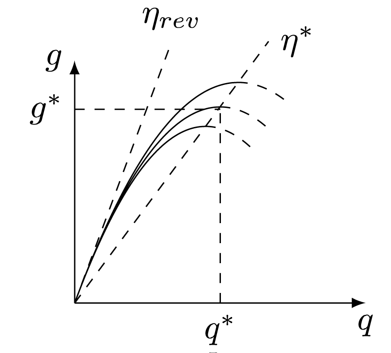
Figure 1: The elements of mobile measuring stands used for powering management and optical communication [18].
satisfy the conditions of the independence from a.
The same conditions are true for those separation processes whose boundary of the realizability domain is determined by (45).
Optimal separation flowsheets
We will take the problem of optimal separation flowsheets as an example of the fact that the efficiency corresponding to the maximum performance does not depend on parameters of the irreversible process.
The energy dissipation increases and the realizability domain becomes narrower when α decreases, but points of the maximum performance and the corresponding heat energy supply stay on the line having the slope .
It is important that if the efficiency of the reversible process for one engine is greater than for another one, the same will be true for both engines for the realizable irreversible process too. Indeed, denoting the ratio of the heat energy supply q and its value corresponding to the maximum power output q∗ as q0 one can get
,
where q0 ∈ [0,1].
This property can be used for solving the problem of choosing the optimal separation flowsheet for the system of two engines using the condition of the minimum overall heat energy supply. The feed flux, its composition and composition of products are given so the separation work A0 is also given. The relation between the efficiency of the reversible process and the irreversible one allows one to choose the optimal separation flowsheet using the condition of the maximum efficiency of the reversible process (minimum heat energy supply for the reversible process).
Components are ordered by the value of some property γ used for the separation (for distillation it is the boiling point temperature). Values γ are normalized to [0,1].
The order of the separation can be of two types:
Direct: the components with γ < γ1 are taken out on the first stage. Components with greater values of γ are separated on the second stage into two products. Components of the first one have γ1 ≤ γ < γ2 and components of the second one have γ ≥ γ2.
Indirect: the component with γ > γ2 are taken out on the first stage. Components wit lesser values of γ are separated on the second stage into two products. Components of the first one have γ1 ≤ γ < γ2 and component of the second one have γ ≤ γ1.
The entropy of flows being separated decreases proportionally to the separation work with the factor RT0 — the product of the gas constant and the temperature of the environment (this factor is included into A below). The decrease of the entropy of the material flow must be compensated by the increase of the heat energy supply flow δsq = q (1/T− − 1/T+) for the reversible process, where temperatures T+ and T− are temperatures of the heat energy supply and outflow respectively. The heat energy flow becomes proportional to the separation work on every stage. The factor of this proportionality is called the temperature coefficient:
.
Temperature coefficients depend on the flowsheet chosen, because the temperatures of the reboiler and the reflux drum depend on the composition of the feed flow and increase monotonously with the increase of γ. This temperatures can be found using the Antoine equation [1]. The overall heat energy supply depends on the flowsheet chosen unlike the overall separation work, because of the existence of temperature coefficients.
Denoting temperature coefficients corresponding to the separation boundaries with γ1 and γ2 as KT1 and KT2 respectively and denoting values of the separation work for the second stage for the direct and indirect order as A21 and A22 respectively one can obtain the overall heat energy supply for both separation orders:
(53)
The sign of the following difference determine the preferred order:
. (54)
The direct order will be preferred if this difference is negative, the indirect one will be preferred otherwise. For the multi-stage system the rule (54) is true for every two subsequent stages.
The expression within brackets are non-negative because it is the separation work per mole of the feed flow. It means that separation boundaries must be chosen such way that temperature coefficients will not decrease from the given stage to the next one.
The feature of the boundary of the realizability domain plotted on the fig. 1 leads to the fact that the flowsheet chosen will be optimal if one consider the irreversible process too.
ConclusionConclusion
References
- Bosnjakovic F. Technical Thermodynamics. Holt, Rinehart & Winston of Canada Ltd. 1965. Ref.: https://goo.gl/jTaCGG
- Green D, Perry R. Perry's Chemical Engineers' Handbook. Eighth Edition. McGrawHill Education. 2007. Ref.: https://goo.gl/nWFaf8
- Tsirlin A. Neobratimye otsenki predelnykh vozmozhnostej termodinamicheskikh i mikroekonomicheskikh sistem (in Russian). Moscow: Nauka. 2003.
- Novikov I. The efficiency of atomic power stations. J Nucl Energy II. 1954; 7: 125-128. Ref.: https://goo.gl/51XW3r
- Dincer I, Rosen M. Exergy. 2nd Edition. Elsevier Science. 2012. Ref.: https://goo.gl/smUXYj
- Salamon P, Nulton J, Andresen B, Roach T, Felts B, et al. Application of finite-time and control thermodynamics to biological processes at multiple scales. J Non-Equilib Thermodyn. 2018; 43: 193-210. Ref.: https://goo.gl/utMwzW
Schwalbe K, Hoffman K. Optimal control of an endoreversible solar power plant. J Non-Equilib Thermodyn. 2018; 43: 255-271. Ref.: https://goo.gl/U1BYbG- Chen L, Yan Z. The effect of heat transfer law on the performance of a two-heat-source endoreversible cycle. J Chem Phys. 1989; 90: 3740-3743. Ref.: https://goo.gl/aobmXC
- Chen L, Sun F, Wu C. Effect of heat transfer law on the performance of a generalized irreversible carnot engine. J Phys D: Appl Phys. 1999; 32: 99-105. Ref.: https://goo.gl/TPhjzT
- Chen L, Li J, Sun F. Generalized irreversible heat engine experiencing a complex heat transfer law. Appl Energy. 2008; 85: 52-60. Ref.: https://goo.gl/3M56Se
- de Vos A. Efficiency of some heat engines at maximum power conditions. Am J Phys. 1984; 53: 570-573. Ref.: https://goo.gl/k4FvND
- Song H, Chen L, Li J, Fengrui Sun. Optimal configuration of a class of endoreversible heat engines with linear phenomenological heat transfer law. J Appl Phys. 2006; 100.
Ref.: https://goo.gl/E8R7RB - Song H, Chen L, Sun F. Endoreversible heat engines for maximum power output with fixed duration and radiative heat-transfer law. Appl Energy. 2007; 84: 374-388. Ref.: https://goo.gl/8astj3
- Song H, Chen L, Sun F, Shengbing Wang. Configuration of heat engines for maximum power output with fixed compression ratio and generalized radiative heat transfer law. J Non-Equilib Thermodyn. 2008; 33: 275-295. Ref.: https://goo.gl/WauJ83
- Li J, Chen L, Sun F. Optimal configuration of a class of endoreversible heat-engines for maximum power-output with linear phenomenological heat-transfer law. Appl Energy. 2007; 84: 944-957. Ref.: https://goo.gl/Q6KPoY
- Chen L, Song H, Sun F, Shengbing Wang. Optimal configuration of heat engines for maximum efficiency with generalized radiative heat transfer law. Rev Mex Fis. 2009; 55: 55-67. Ref.: https://goo.gl/wFkffM
- Ares De Parga G, Angulo-Brown F, Navarrete-Gonzalez T. A variational optimization of a finite-time thermal cycle with a nonlinear heat transfer law. Energy. 1999; 24: 9971008. Ref.: https://goo.gl/LSv2Q4
- Ait-Ali M. The maximum coefficient of performance of internally irreversible refrigerators and heat pumps. J Phys D: Appl Phys. 1996; 29: 975-980. Ref.: https://goo.gl/AX4LNJ
- Rozonoer L, Tsirlin A. Optimal control of thermodynamic processes i-iii. Autom Remote Control. 1983; 44: 314-326. Ref.: https://goo.gl/4p6Hex
- Tsirlin A, Sukin I. Finite-time thermodynamics: The maximal productivity of binary distillation and selection of optimal separation sequence for an ideal ternary mixture. J Non-Equilib Thermodyn. 2014; 39: 13-25. Ref.: https://goo.gl/mg5uJE
- Tsirlin A, Sukin I. Attainability region of binary distillation and separation sequence of three-component mixture. Theor Found Chem Eng. 2014; 48: 764-775. Ref.: https://goo.gl/bERV7e